Introduction · Written before the mathematical derivations
Companion video: E09 “The Tail End of Berlin · 1753–1766”
To be honest, after I finished making this episode’s video, one thing stayed with me strongly: in the 15 years from 1750 to 1765, Euler, alone at his desk in Berlin, had 4 notebooks open at the same time. Looking back now, what was written in those 4 notebooks grew, respectively, into today’s topology, computational fluid dynamics, attitude control, and internet cryptography.
In the video we only had time to tell the story and give the intuition; the part about “why it really holds” has to be written down here… My own feeling is that for many viewers, just watching the video is not enough; they will feel “Euler was really impressive, but I still don’t know how it actually works”. So there is this blog post.
Below I will use roughly 5 minutes’ worth of space to say what each of the 4 theorems is about, and why they are still being used 270 years later. It is fine to stop once you have read that far; if you want to go on to the proofs, scroll down to §1 through §4.
The 4 mathematical stories of this episode
§1 · V − E + F = 2 — the polyhedron identity
A cube has 8 vertices, 12 edges, 6 faces: 8 − 12 + 6 = 2. A regular tetrahedron: 4 − 6 + 4 = 2. On November 14, 1750, Euler wrote to Goldbach and stated this for the first time.
Why? Because a polyhedron’s “freedom of shape” and its “surface topology” are two different things… however you squeeze it and however you stretch it, as long as you do not poke a hole, this 2 will not change. This one observation later became the starting point of all of topology.
One application I personally found rather surprising is the soccer-ball molecule C60. In 1985 chemists discovered that carbon atoms have a configuration in which exactly 60 atoms form a soccer ball; this kind of molecule is called a fullerene. Euler’s formula here forces it to have exactly 12 pentagonal faces — not one more, not one less, and this has nothing at all to do with how many hexagons there are. In 1996 this discovery won the Nobel Prize.
§2 · The fluid equations — the first partial differential equations
When Newton wrote F = ma it was meant for “point masses”. But what about water? What about air?
From 1752 to 1755, Euler extended F = ma to continuous matter… and the result was the first system of partial differential equations in human history. Today this set of equations goes by the name CFD; airplane wings, weather forecasting, simulations of blood flow in the heart all use it.
Its extended version, Navier-Stokes, is still one of the 7 Millennium Prize Problems, with a prize of 1 million US dollars; the reward has been offered for 25 years and no one has been able to solve it. Our understanding of how fluids behave is still incomplete today.
§3 · The rigid-body equations + Euler angles — why a top does not fall over
The Earth spins about its axis once every 24 hours; the front wheel of a bicycle, when it spins fast, does not fall over; a nut floating freely on the ISS spontaneously flips over periodically… These seemingly unrelated phenomena are all described in one sentence by Euler’s rigid-body equations .
That 1985 Dzhanibekov nut experiment on the Salyut 7 space station is very striking, compared with the ground, where this phenomenon simply cannot be seen. Today the attitude control of flying vehicles, the planning of robot wrists, and the algorithms that rotate bones in animation engines all rest, at the bottom, on this mathematics that Euler ground out over 15 years in Berlin.
§4 · Euler’s theorem + RSA — the root of contemporary cryptography
In 1763 Euler generalized a small observation of Fermat’s (“2 to the 6th power equals 64, which leaves remainder 1 when divided by 7”) to an arbitrary modulus.
213 years later, in 1977, three people at MIT — Rivest, Shamir, Adleman — discovered that this theorem of Euler’s could be used to build a kind of asymmetric encryption. The key used for encryption can be made public, while the key for decryption is kept strictly secret… This is RSA.
What I find interesting when I think about it is that when Euler was writing this theorem, he could not possibly have foreseen that centuries later it would become the cornerstone of the whole internet’s system of trust. Today the padlock in your browser’s address bar, the login to your banking app, every encrypted email you send — the first step, the handshake, uses RSA.
Why put these 4 theorems in one episode?
They look as though they have nothing whatsoever to do with each other — topology, fluids, rigid bodies, number theory. But they were written by the same person, in the same period, in the same city, at the same desk. 1750 to 1765: Euler’s 15 years in Berlin.
Thinking back on the popular introductions to Euler I used to read, they generally say “he researched everything”, “he was the king of mathematics”; this kind of description is actually of no use, and after hearing it you know nothing. I myself tend to think of it this way: in those 15 years he did not know that these 4 things would become the foundations of 4 modern disciplines; he just spread 4 notebooks out on his desk and wrote at his own pace. Looking back today, each one of these 4 notebooks has grown into a large tree.
The 4 §s below are complete, peer-reviewed, rigorous proofs. Every formula is derived from the beginning. If at any point you feel “wait, why is this so”, you can go back to the corresponding timecode in the video (marked at the top of each §), or look directly at the worked example block and compute it once with concrete numbers — I think that for many people, computing it once with concrete numbers is easier to understand than reading an abstract proof.
By the way, this blog post was actually not written by me alone. The proofs were written by Abel, Socrates and Gauss each did two rounds of review (logical rigor + historical fact-checking), Escher made the illustrations and GIF animations, and Euler handled the Ghost publishing. My own part is this introduction, plus steering the direction of the whole project. I find this way of collaborating quite novel… one person plus a group of AI partners, each with their own specialty, produces something that is probably a good deal more rigorous than what I would write on my own.
— Yeqiu and his AI partners · timeobserver137
§1 · Rigorous proof of the polyhedron formula V−E+F=2
Companion video: 04:07–07:40 (segment M1)
This section assumes you are familiar with
: high-school solid geometry (counting vertices/edges/faces), elementary graph theory (vertices, edges, faces, connectedness), induction.
Summary in one sentence
For any convex polyhedron (more generally, for any finite polyhedron homeomorphic to the sphere), the number of vertices , the number of edges and the number of faces always satisfy
This identity was put forward by Euler in a letter to Goldbach on November 14, 1750. On the surface it is an elementary combinatorial equation, but in fact it is the first cornerstone of topology: today we call the quantity the Euler characteristic of the surface, and for the sphere . This section gives four routes of proof from 1750 to the modern day, highlighting the assumptions and gaps of each step.
1.1 Euler 1750: the informal cut-a-face-and-flatten argument
The argument Euler himself gave runs roughly as follows:
Step 1: Take any face of the polyhedron and “cut out” that face, obtaining a polyhedral shell with a hole; at this point and are unchanged and decreases by 1, so
Step 2: Flatten the remaining shell onto the plane along the boundary that was cut out. After flattening one obtains a plane graph , still with vertices and still with edges, and with bounded faces plus unbounded outer face, in total.
Step 3: Repeatedly apply two kinds of reduction to the plane graph: - Triangulation: if some bounded face is not a triangle, add a diagonal inside it; and each increase by , and the identity is unchanged. - Deleting an edge or a vertex: when all faces are already triangles, deleting a boundary triangle correspondingly decreases and each by (or, removing a leaf vertex, decrease together), and the identity is unchanged.
Step 4: Keep reducing until only one triangle is left, (one triangular face + one outer face); at this point . Tracing back through all the reductions, the original polyhedron also satisfies .
Gaps: Euler’s argument has two non-rigorous points, which it took later generations more than 60 years to fill.
- Flattening does not always give a plane graph: the geometric action of “unfolding the shell onto the plane” is shape-preservingly feasible only for convex polyhedra; for a non-convex polyhedron (such as a star shape with grooves) one must first argue that it can be deformed homotopically and continuously to the sphere and then flattened. Euler tacitly assumed the polyhedron was convex, but he did not say so explicitly.
- Convergence of the triangulation–edge-deletion reduction: does this process terminate for an arbitrary plane graph? Euler assumed one could delete all the way down to a single triangle, but whether it could fall into an infinite loop (for example, all faces are triangles but there is no boundary triangle that can be deleted) was not proved.
These two gaps were filled by Legendre in 1794 and Cauchy in 1813 respectively.
1.2 Legendre 1794: the spherical excess route
Core idea: Inscribe the convex polyhedron in the unit sphere, and project each face of the polyhedron from the center of the sphere. Each face becomes a spherical polygon, and all the faces of the polyhedron cover the whole sphere, with total area .
Lemma (spherical triangle formula). For a triangle on the unit sphere whose three interior angles are , its spherical area satisfies
(This is the famous result of Harriot 1603 / Girard 1629; the area of a general spherical -gon is its interior angle sum minus .)
Corollary (spherical -gon). The spherical area of an -gon on the sphere is
Outline of Legendre’s proof.
Let the -th face project to a spherical -gon, with interior angle sum and number of edges . All the faces cover the total area of the sphere:
Next, count each term separately:
- counts the sum of the numbers of edges of each face. But each edge belongs to exactly two faces, so .
- is the sum of the interior angles of all faces at all vertices. At each vertex, the sum of the interior angles of all the spherical polygons having that vertex as a corner is exactly (they go around that point on the unit sphere one full turn). So .
Substituting gives
Advantage: this proof completely avoids Euler’s flattening action, using only spherical geometry and simple counting; its drawback is that it applies only to convex polyhedra (only these can be inscribed in a sphere and projected from the center).
1.3 Cauchy 1813: the modern textbook standard (induction on plane graphs)
In Recherches sur les polyèdres, Cauchy gave the earliest inductive proof that is rigorous in the strict sense; it is also the version most commonly used in modern graph theory and topology textbooks.
First step: Following Euler’s 1750 line of thought, choose a face, cut it out and flatten into a plane graph . We want to prove that every connected plane graph satisfies
where includes the unbounded outer face (that is, the unbounded region corresponding to the face that was cut out).
Second step (base of induction): the single-point plane graph (only one outer face); obviously .
Third step (induction): For any connected plane graph (number of vertices ), split into two cases, “contains a cycle vs. tree”:
- Case A: contains a cycle. Pick any edge lying on the cycle and delete it. After deletion the graph is still connected (removing one edge from a cycle, other paths take its place), is unchanged, decreases by ; and the two faces that separated in the original graph merge into one, so also decreases by . By the induction hypothesis , so .
- Case B: contains no cycle (that is, is connected and acyclic, a tree). Any tree with vertices contains at least two leaf vertices (vertices of degree ). Choose one leaf vertex and its unique incident edge , and delete them together → decreases by , decreases by , is unchanged (a tree originally has only outer face, and deleting a leaf neither adds nor removes faces). By the induction hypothesis .
(Note: the originally naive assertion “if is a bridge, then one of its endpoints must be a leaf” is in fact not true — a counterexample is the barbell graph (a bridge edge between two triangles), where both ends of the bridge have degree . The corrected “contains a cycle vs. tree” dichotomy is universal and rigorous.)
By induction, every connected plane graph satisfies .
Key observation. Cauchy’s proof depends only on the connectedness and planarity of the graph, not on geometric convexity. It therefore extends Euler’s formula in one stroke from convex polyhedra to any polyhedron homeomorphic to the sphere (allowing Schönhardt-type ones that are non-convex but topological spheres).
Pitfall: this proof does not tell us how the formula should be corrected once a polyhedron is no longer homeomorphic to the sphere (for example a torus with a handle). That had to wait until Riemann (1851) and Poincaré (1895) provided a new language.
1.4 The modern view: the topological invariant
At the beginning of the 20th century, topologists discovered that is not only a numerical identity but a homotopy invariant of a simplicial complex.
Definition. For a compact connected 2-dimensional manifold , choose any simplicial subdivision of it (that is, cut into finitely many triangles, such that adjacent triangles share an edge or a vertex); let the triangulation have vertices, edges and (triangular) faces, and define
Core theorem. does not depend on the particular subdivision; it depends only on the homeomorphism type of .
Examples: - The sphere : . - The torus (doughnut): . - The genus- orientable closed surface : . - The Klein bottle: . - The projective plane : .
This restates Euler’s formula as a clean topological criterion (forward direction):
(The reverse direction also holds, but it requires the classification theorem for compact 2-dimensional manifolds (from Möbius/Klein/Dyck 1888 on); see Massey Algebraic Topology §I.7 or a similar textbook; this section does not go into it.)
Geometric intuition. The surface of a convex polyhedron is homeomorphic to the sphere (radial projection is a homeomorphism), so , which is equivalent to . If the surface of the polyhedron is allowed to “grow holes” (such as a torus-type polyhedron with a handle), then no longer equals but .
Independent of stretching/bending. is a homeomorphism invariant, which means that however the surface is continuously deformed (without tearing or gluing), the value of does not change. This is the first clear example of “topology does not depend on metric”.
Worked examples
Example 1: verifying the count for the octahedron
The regular octahedron has vertices (the top and bottom apexes + the 4 vertices of the middle square), edges (the top and bottom apexes each connect to the 4 square vertices = 8 + the 4 sides of the square = 12), triangular faces (4 on the upper pyramid + 4 on the lower pyramid).
What this tells us: the surface of the regular octahedron is homeomorphic to the sphere; it is a topological sphere with .
Example 2: verifying the truncated icosahedron (soccer ball)
The modern soccer-ball pattern is the truncated icosahedron: shave a triangle off each of the 12 vertices of the regular icosahedron, obtaining 12 pentagons (shaved from the vertices) + 20 hexagons (turned out of the original 20 triangular faces).
- Number of vertices (each original vertex shaved yields 5 new vertices, )
- Number of edges (12 pentagons + 20 hexagons, each edge belongs to two faces, — wait, recompute: pentagons 5 edges × 12 = 60, hexagons 6 edges × 20 = 120, total edge count (with repetition) = 180, each edge counted twice, ✓)
- Number of faces
What this tells us: even for a fairly complex polyhedron with a “non-convex feel” (in fact the Carbon 60 fullerene also has this shape, chemistry 1996, the Kroto-Smalley-Curl Nobel Prize), as long as it is topologically a sphere, always = 2. This is why all the fullerene (buckyball) molecules discovered in 1985 must contain exactly 12 pentagons — solving + + simultaneously gives , independent of the number of hexagons .
Geometric/physical intuition
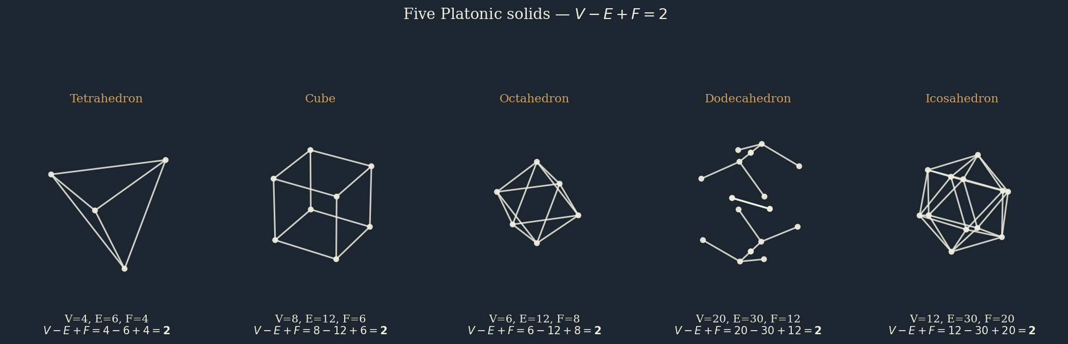
Fig 1.
Wireframe projections of the five Platonic solids + V/E/F counts. χ = V−E+F = 2 holds identically on all five surfaces.
🎬 Visualization of the cut-flatten proof — video 06:24 (anim-04): remove one face, flatten the remaining network onto the plane, inductively delete edges/vertices → proving V−E+F = 2 (chunk M1_07).
🎬 Sphere ↔ torus homotopic deformation — video 06:00 (anim-03): comparison of the topological invariant χ=2 (sphere) and χ=0 (torus) (chunk M1_06).
Imagine the polyhedron as an inflated rubber ball: the vertices are markers, the edges are rubber bands, the faces are rubber membranes. However you squeeze, stretch, twist this ball, as long as you do not puncture it and do not glue two membranes together, the combined value of the number of vertices, edges and faces is always .
But once you poke a hole and turn it into a doughnut (torus), immediately jumps to , and this has nothing at all to do with how you “draw” the edges or how you divide the “faces” — it is an innate global property of this surface, independent of the subdivision.
Video correspondence
Video 04:07–07:40 (segment M1): - 04:07–04:38: the Goldbach letter + V−E+F=2 surfaces for the first time (anim-20) - 04:40–05:09: V/E/F letter hover + tetrahedron 4 vertices 6 edges 4 faces counter (anim-01, anim-21) - 05:10–05:35: 5 regular polyhedra verify V−E+F=2 (anim-02) - 05:35–06:05: sphere ↔ torus homotopic deformation, jumps from 2 to 0 (anim-03) - 06:05–06:35: visualization of Euler’s 1750 cut-face–flatten proof (anim-04) - 06:35–07:10: 200-year topology relay portrait grid: Cauchy 1813 / Riemann / Poincaré 1895 / Perelman 2003 (anim-05)
— Abel
§2 · From Newton to Euler: deriving the equations of fluid motion
Companion video: 07:45–11:11 (segment M2)
This section assumes you are familiar with
: multivariable calculus (partial derivatives, chain rule), vector calculus (gradient , divergence ), the divergence theorem (the Gauss-Ostrogradsky formula), Newton’s second law.
Summary in one sentence
Between 1752 and 1755, Euler extended Newton’s second law from discrete “point masses” to a “continuous medium” (that is, assuming that a fluid can be regarded as a continuous field of matter, with a well-defined local density and velocity at any scale — also called the continuum hypothesis, not to be confused with the set-theoretic proposition of the same name). This extension produced the first genuine system of partial differential equations — the Euler fluid equations:
It translates “force = mass × acceleration” into the language of vector fields, and is still the cornerstone of computational fluid dynamics (CFD) today. This section gives the standard derivation starting from a control volume, and then briefly introduces how Navier 1822 and Stokes 1845 added the viscous term and extended it into the Navier-Stokes equations.
2.1 The material derivative: the acceleration following a fluid element
Problem. In a continuous medium, the velocity field gives the fluid velocity at spatial position at time . But Newton’s second law concerns the acceleration of a particular fluid element, not the acceleration at a point in space. The two are not the same.
Key distinction: - Eulerian view: observe at a fixed spatial point how the velocity changes. is the time variation of the velocity at a fixed point in space. - Lagrangian view: follow the motion of a particular labeled fluid element. In , the is that element’s “own acceleration”.
Lemma (material derivative). The acceleration following the motion of a fluid element can be written as
Proof. Let the fluid element at time be located at , with velocity . By the chain rule,
And (the element is simply carried along by the velocity field), so
Intuition. The first term is the local time variation (if you stand on a fixed riverbank, how the speed of the river water changes); the second term is the convective term (if you sit in a small boat, the change in velocity you feel as you drift with the river to different places). Only the sum of the two is the acceleration the fluid element itself feels.
2.2 Newton’s second law + control volume → the Euler equations
Core idea. For a fluid element of density and volume , Newton’s second law is written as
We need to write the on the right as the sum of the various kinds of force.
Three kinds of force acting on the element:
- Pressure gradient (surface force): on the 6 faces of the element, each face bears the pressure of the surrounding fluid. Let the element be a box with sides ; the pressure difference between the left and right faces along the direction is
The same holds in all three directions, and the resultant force is .
- Gravity (body force): the weight of the element is .
- (Viscous force ignored for now): the core assumption of Euler’s model is an inviscid fluid — there is no internal friction between fluid elements, which interact only through pressure. Formally, this is equivalent to asserting that the Cauchy stress tensor is isotropic:
That is, the stress on any small fluid surface consists only of the normal pressure , with no shear stress (the off-diagonal for are all ). This is the biggest gap from reality, later filled by Navier and Stokes (see 2.4) — the of a Newtonian fluid contains shear terms linear in the strain rate.
Total resultant force:
Substituting into Newton’s second law (dividing both sides by ):
This is the Euler fluid momentum equation (Euler equation of motion; 1755 Principes généraux manuscript / 1757 published in the Mémoires de l’Académie de Berlin).
🎬 Fluid element force balance — video 08:44 (anim-06): balance of 3 forces on a fluid element (pressure gradient / body force / acceleration) + building the Euler equation, chunk M2_03.
Worked example: incompressible ideal flow around a stationary sphere — the surface pressure distribution
Consider a uniform flow of speed flowing past a stationary sphere (radius ), assuming inviscid + incompressible + irrotational. The velocity field outside the sphere is known (from the Laplace equation + Neumann boundary conditions, e.g. Lamb Hydrodynamics):
Apply the formula (Bernoulli along a streamline). For a steady ideal flow, along any streamline . Take the reference point at infinity (, ):
Compute (on the sphere ):
What this tells us: on the sphere, the pressure is greatest at (the stagnation point facing the flow, the “nose”) and at (the rear stagnation point) ( above ambient pressure); on the two sides of the sphere () the pressure is smallest ( below ambient).
Note: a pressure distribution symmetric front to back means that the net drag of inviscid flow around a sphere — the famous D’Alembert paradox (1752). The drag of real fluids comes from the viscous term added in §2.4; this is the core limitation of the Euler equations.
2.3 Conservation of mass → the continuity equation
Problem. For each fixed spatial region , how does the total mass inside the region change over time?
Principle of conservation of mass: change of mass inside the region = inflow - outflow.
Formalization. The total mass inside region is
The mass flow rate out through ‘s boundary is
where is the outward unit normal vector on . Conservation of mass is then
The divergence theorem (Gauss / Ostrogradsky) converts the boundary integral into a volume integral:
Substituting and exchanging integration and differentiation (for a fixed region , can be moved inside the integral):
Key (du Bois-Reymond vanishing lemma): this holds for any region . Assume the integrand is continuous; if at some point we have (without loss of generality ), then by continuity there exists around a neighborhood such that on all of ; taking gives , a contradiction. So the integrand is everywhere:
This is the continuity equation, which turns conservation of mass from an integral form into a partial differential equation.
Special case: incompressible flow. If , then and , and the continuity equation simplifies to
This is the standard assumption for water flow, and for air at low speeds.
Worked example: incompressible flow through a pipe of varying cross-section
Consider water (incompressible) flowing through a pipe, with inlet cross-section radius and inlet velocity . The pipe narrows to an outlet radius . Find the outlet velocity .
Apply the formula: for steady incompressible flow, together with the pipe wall not leaking (that is, conservation of volume flow rate) gives
Compute:
What this tells us: halve the radius and the velocity becomes times as large — the continuity equation translates “conservation of mass” into the everyday intuition “the pipe narrows, the flow speeds up” (this is the principle behind squeezing the outlet of a garden hose: the jet of water gets thinner but flies farther).
🎬 Continuity equation inflow/outflow + density change — video 09:22 (anim-07, chunk M2_04). 🎬 ODE → PDE bridge metaphor — video 09:43 (anim-25, chunk M2_05): an intuitive bridge for understanding a “single-point ordinary differential equation” as a “partial differential equation over a whole continuous medium”.
2.4 Navier 1822 + Stokes 1845: adding the viscous term
The core defect of the Euler equations is the assumption of inviscid flow, but real fluids have friction at the molecular scale inside them. Navier (1822) and Stokes (1845) each independently added the viscous force to the Euler equations.
Core idea. The viscous force comes from velocity gradients inside the fluid — adjacent layers of flow produce shear stress because of their difference in velocity. In the framework of the Cauchy stress tensor, for a Newtonian fluid (stress linear in strain rate),
where is the shear viscosity coefficient and is the bulk viscosity coefficient.
For incompressible flow (), the divergence of the stress above simplifies to , and substituting into Newton’s second law gives
where is the kinematic viscosity. These are the Navier-Stokes equations for an incompressible Newtonian fluid.
Relation to the Euler equations: taking the limit returns the Euler equations, so the Euler equations are the N-S equations in the ideal / inviscid case.
🎬 Euler → Navier-Stokes formula evolution — video 10:27 (anim-09): adding the viscous term ν∇²v to the right side of the Euler equation evolves it into the NS equations, chunk M2_07.
Worked example: Poiseuille laminar flow in a circular pipe — an analytic solution of NS
Consider steady, incompressible, axisymmetric laminar flow through a circular pipe of radius and length , with a pressure difference between the two ends. Find the velocity distribution and the total flow rate .
Modeling assumptions: - Steady: - Axisymmetric: (flow only in the direction, varying only with ) - Incompressible: ✓ (automatic) - No gravity (horizontal pipe), or gravity along the axis absorbed into
Simplifying the NS equations. The convective term ( does not depend on ). The -direction NS:
In cylindrical coordinates with axial symmetry, . The -direction NS gives , that is, . The -direction pressure gradient is constant: . Substituting:
Integrate (using ):
Since the velocity is finite at . Integrating again:
From no slip at the pipe wall, . Finally:
Total flow rate:
What this tells us: the velocity distribution is a parabola (fastest on the axis, zero at the wall); the flow rate — double the radius and the flow rate becomes 16 times as large! This is why hardening of the arteries in the human body (blood-vessel radius reduced by 20%) increases the burden on the heart (the pressure difference) several times over. Poiseuille’s experiments of 1838-46 measured this formula; it is the first engineering-grade law in fluid mechanics derived rigorously from the NS equations.
Historical timeline: - 1752-08-31: Euler submits Principia motus fluidorum (E258), giving the 2D incompressible flow equations for the first time. - 1755 / E226: Principes généraux du mouvement des fluides, the complete 3D generalization. - 1822: Claude-Louis Navier adds the viscous term (but his derivation, based on molecular assumptions, is disputed). - 1845: George Gabriel Stokes re-derives it using the continuum stress tensor, giving today’s textbook form.
A current world-class open problem: global well-posedness of NS (Clay Millennium Problem). For general 3D initial data, can the existence + uniqueness + smoothness of NS solutions be established on arbitrary time intervals? This is one of the 7 Millennium Prize Problems, with a prize of 1 million US dollars. As of 2025, the main progress is the 1982 Caffarelli-Kohn-Nirenberg estimate of the Hausdorff dimension of the singular set of suitable weak solutions, but a complete answer has still not been given.
2.5 Vorticity and Helmholtz’s vortex theorems (supplement)
Define the vorticity . Taking the curl of the Euler equation gives the vorticity equation
which reveals Helmholtz’s three vortex theorems of 1858: vortex lines move with the fluid elements, vortex lines have no endpoints, and the strength of a vortex tube is conserved over time. This is the theoretical basis for the analysis of atmospheric circulation, tornadoes, and wing lift.
🎬 Kármán vortex street — video 10:02 (anim-08): periodic shedding of the vortex row behind a cylinder + visualization of vorticity ω = ∇×v, chunk M2_06.
Geometric/physical intuition
Imagine the fluid as a pot of little water droplets pushing against each other. The left side of the Euler fluid equation
is “the acceleration of a particular droplet”. The right side is the force this droplet bears: - : the high-pressure region pushes it toward the low-pressure region (pressure gradient). - : gravity.
The continuity equation
is “droplets do not vanish or appear out of nowhere in a region” — the local density can change only because matter flows in or out.
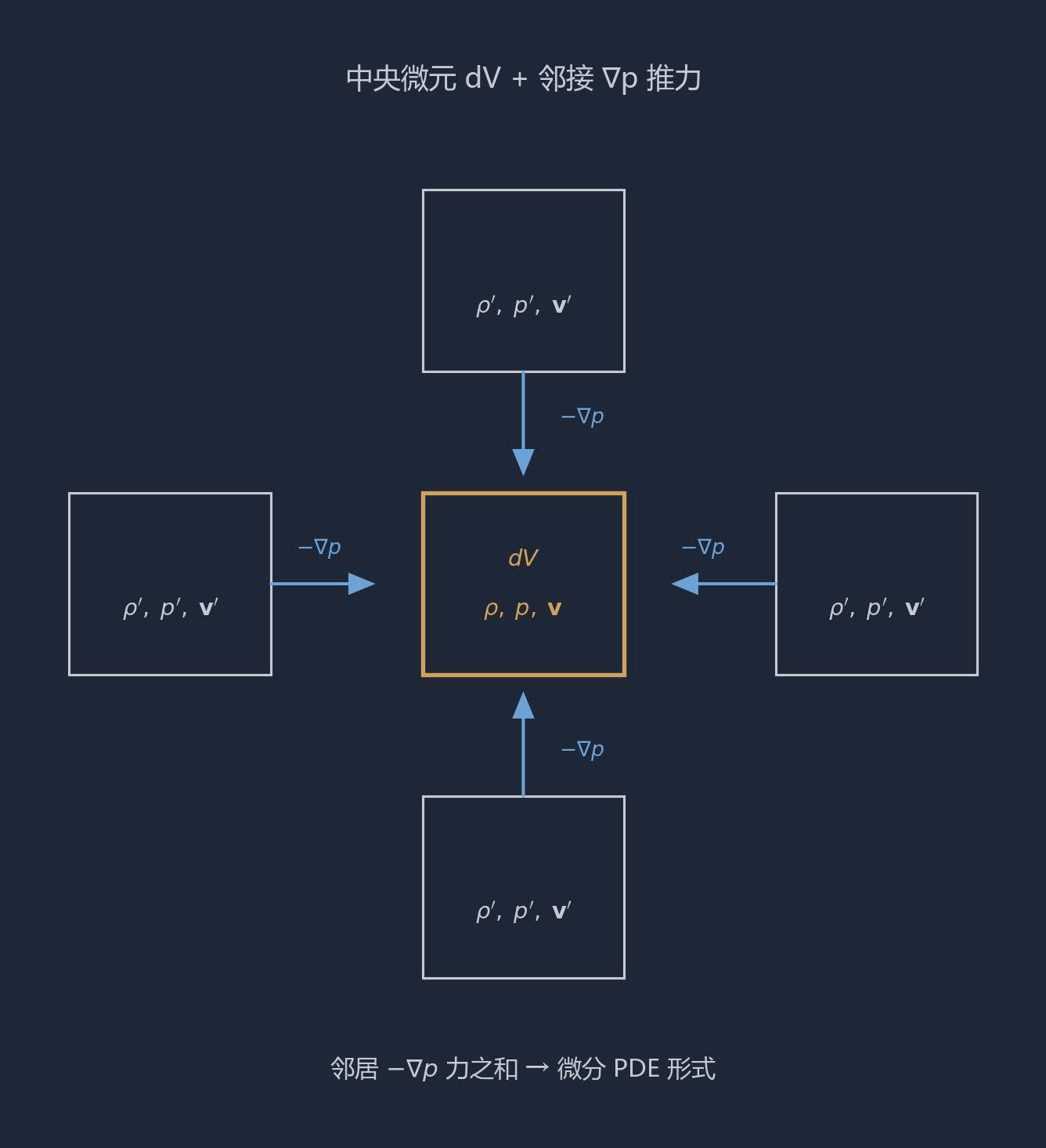
Fig 2.
A central fluid element + 4 adjacent elements (up / down / left / right) + inward pressure-thrust arrows. The inside of the element is described by three state quantities (ρ, v, p); the neighbors are coupled, in the form of a pressure gradient, to the −∇p/ρ term on the right side of the central equation. This is a geometric miniature of the continuum hypothesis.
Video correspondence
Video 07:45–11:11 (segment M2): - 07:45–08:15: single-point particle → continuous medium expand (anim-23) - 08:15–09:00: material derivative + Euler eq force balance (anim-06) - 09:00–09:35: continuity equation inflow/outflow (anim-07) - 09:35–10:10: ODE→PDE bridge metaphor (anim-25) - 10:10–10:40: continuum PDE buildup, momentum + mass (anim-24) - 10:40–11:11: Euler → Navier-Stokes evolution + Karman vortex street (anim-09, anim-08)
— Abel
§3 · The rigid-body equations and Euler angles
Companion video: 11:16–14:51 (segment M3)
This section assumes you are familiar with
: multivariable calculus (chain rule, partial derivatives), linear algebra (eigenvalues of real symmetric matrices and the spectral theorem), vector analysis (cross and dot products, matrices).
Summary in one sentence
In 1765, in Theoria motus corporum solidorum seu rigidorum (published in Rostock+Greifswald), Euler systematically synthesized Newton’s into the equations of rotational motion of a whole rigid body, obtaining the famous Euler rigid-body equations
where is the angular velocity vector, is the inertia tensor, and is the external torque.
But this theory did not suddenly pop up in 1765 — it was Euler’s accumulation across 15 years:
- 1750-09-03: Découverte d’un nouveau principe de mécanique (E177) — the first version of the rigid-body equations
- 1751: the body-fixed frame turned into a tool
- 1758: Recherches sur la connoisance mechanique des corps (Berlin Mémoires) — discovery of the principal axes of inertia + the first appearance of the term “moment of inertia”
- 1765: Theoria motus — the synthesized system
The key to the whole theory is the introduction of the inertia tensor + the parametrization of SO(3) by Euler angles (φ, θ, ψ), and the proof of Euler’s rotation theorem: any rotation in three-dimensional space can be expressed as a rotation about some instantaneous axis. This section gives the tensor framework of , the body-frame derivation of the rigid-body equations, the geometry of 3-1-3 Euler angles, and the SO(3) eigenvalue proof of the rotation theorem.
3.1 Angular momentum and the inertia tensor
Definition (rigid body). A body made up of finitely many (or continuously distributed) point masses, in which the distance between any two point masses does not change over time.
Angular momentum. Choose a fixed reference point in space (the origin of an inertial frame), and assume that the rigid body rotates relative to (that is, is on the rigid body, or is the fixed point about which the rigid body performs pure rotation). The angular momentum of the rigid body is the sum of the angular momenta of the point masses:
where is the position vector of the -th point mass relative to , and is its velocity.
Key fact. For a rigid body rotating about (angular velocity ), the velocity of each point mass is ; substituting gives
By the BAC-CAB identity :
Writing this in component form (Einstein summation convention) gives
For a continuous mass distribution:
is a symmetric tensor. This is obvious from the definition . Physically, maps the angular velocity vector to the angular momentum vector; it takes over the role of the “scalar inertia” in .
Key property. Since is real symmetric, by the spectral theorem can be diagonalized: there exists an orthogonal basis such that
These three are called the principal axes of inertia, and the three are the principal moments of inertia (for a general mass distribution ; degenerate cases such as a thin rod or a point mass allow some ). This was introduced by Euler in 1758 in Recherches sur la connoisance mechanique des corps (Berlin Mémoires) — which is also the paper in which the term “moment of inertia” first appeared — and was fully retained in the synthesis of the 1765 Theoria motus.
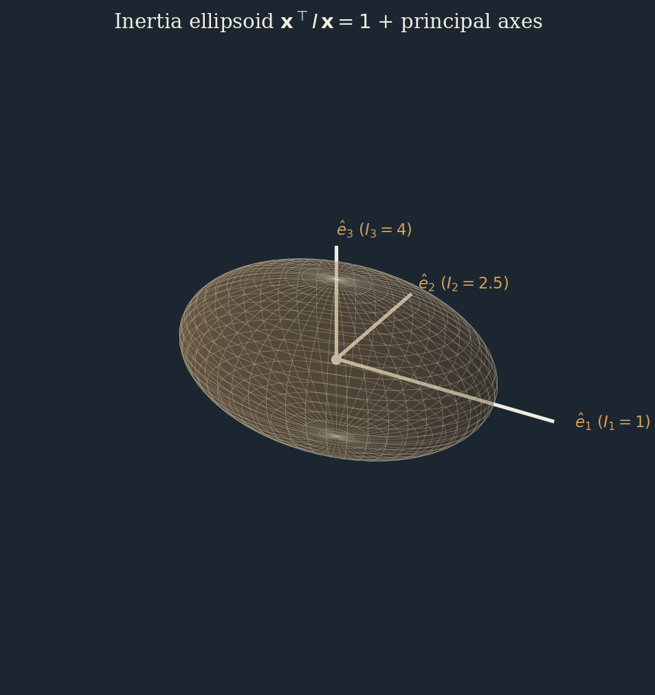
Fig 3.
The inertia ellipsoid — the semi-axis lengths are inversely related to the three principal moments of inertia . The 3 arrows are the directions of the principal axes. Every rigid body, even one of irregular shape, corresponds to a unique inertia ellipsoid.
Worked example: the moment of inertia of a cube about a face-center axis vs a body-diagonal axis
Consider a solid cube with side , uniform density and total mass . Find the moment of inertia (a) about a face-center axis (passing through the centers of two opposite faces) and (b) about a body-diagonal axis (passing through two opposite vertices).
(a) Face-center axis (e.g. the axis, along one of the cube’s symmetry center lines).
By symmetry, the principal axes lie along the three face-center axes, and the principal moments of inertia are .
By symmetry, , so
(b) Body-diagonal axis.
In the face-center-axis basis the inertia tensor is (isotropic, three equal eigenvalues), so is in any orthogonal basis — including the direction of the body-diagonal axis.
What this tells us: because of its cubic symmetry (3 axes + 4 body-diagonal axes), the cube’s inertia tensor is isotropic (degenerate, a triple eigenvalue). About any axis through the center, the moment of inertia is . This is an example of high symmetry “promoting” the principal moments of inertia to a constant. By contrast, a rectangular box (with unequal sides) has three different principal moments of inertia, and its rotational behavior is very different (e.g. the Dzhanibekov effect, see the example below).
3.2 Euler’s rigid-body equations (body-frame derivation)
The rotational version of Newton’s second law (in an inertial frame):
Difficulty. With in the inertial frame, changes over time (because the rigid body is rotating, the orientation of its principal axes is rotating too), and computing is troublesome.
Solution. In the body frame that rotates together with the rigid body, is a constant tensor (the principal axes stay aligned with the body axes). But the body frame is not an inertial frame, so the transformation formula for a rotating reference frame is needed.
Lemma (derivative formula for a rotating coordinate system). For any vector ,
(This is the standard formula for the transformation of velocities in any rotating reference frame — the geometric source of what physics calls the “Coriolis formula”.)
Applied to :
Substitute , with constant in the body frame:
Combined with Newton’s second law :
These are the Euler rigid-body equations, written in the body frame; the three equations correspond respectively to the principal-axis directions.
Component form (along the principal axes):
🎬 Euler rigid-body equations 3-step build — video 12:59 (anim-12): three-step Replacement Transform derivation of I dω/dt + ω×(Iω) = τ, chunk M3_05.
Free rigid body (no external torque) : even with no external force, is not constant — the nonlinear coupling terms such as make the angular velocity “drift” between the principal axes. This leads to free precession and the famous Dzhanibekov effect (the intermediate axis theorem: rotation about the intermediate principal axis is unstable).
Worked example: the Dzhanibekov intermediate-axis effect
Let the rigid body’s principal moments of inertia satisfy (e.g. a box with unequal sides: units). When a free rigid body () rotates about the intermediate axis , give it a tiny perturbation . The Euler equations (no external force):
Linearize (set , with small quantities):
Second-order ODE: .
Stability test. Let , .
- If rotating about the smallest or largest principal axis ( replaced by or ), then the coefficient is a product of a negative and a positive number → → purely imaginary → stable (periodic wobble).
- If rotating about the intermediate principal axis (): , , the product is → → real → exponential growth → unstable.
What this tells us: when a free rigid body rotates about the principal axis of “intermediate inertia”, any tiny perturbation is amplified exponentially, causing the “flip effect” — what looks like a periodic 180° flip is in fact going through a complete exponential–saturation–decay cycle.
The 1985 Dzhanibekov experiment: the Soviet cosmonaut Vladimir Dzhanibekov, on the Salyut 7 space station, unscrewed a wing-nut and let it float and spin freely — the nut spontaneously flipped over periodically, astonishing ground control. This effect could already be predicted within the framework of Euler’s 1758 Recherches (linearization gives it directly), but because gravitational disturbances on Earth are too large, no one had ever seen it on the ground; only in the true weightlessness of space did it show itself. Video: search “Dzhanibekov effect ISS”.
3.3 Euler angles (3-1-3 convention)
Problem. SO(3) (the 3D rotation group) is a 3-dimensional manifold, and 3 parameters are needed to parametrize it locally. Euler angles (φ, θ, ψ) are the classic choice.
3-1-3 convention (z-x-z, the most commonly used in classical mechanics):
Rotate the body frame out of the space frame , in 3 steps in all:
- About , rotate by angle : called precession. .
- About the new (after step 1, called the line of nodes), rotate by angle : called nutation. .
- About the new (the final body z-axis), rotate by angle : called spin. .
The corresponding rotation matrix (in column-vector form):
where
The angular velocity expressed in Euler-angle components (in the body frame):
(These formulas were given in Euler’s 1750 letter + the 1765 Theoria motus, with the 1758 Recherches in between providing the principal-axes framework.)
Singularity (gimbal lock). When or , and cannot be told apart independently — the first and third steps rotate about the same axis. This is a geometric defect of the 3-1-3 parametrization, which in the attitude control of flying vehicles is avoided by switching to quaternions (Hamilton 1843).
Worked example: steady precession of a gyroscope
Consider a pendulum gyroscope toy (a toy top): mass , distance from the center of mass on the spin axis to the pivot point , moment of inertia about the spin axis , spin angular velocity . Find the steady precession angular velocity .
Apply the formula. In the “fast top” approximation, where the spin angular velocity is much larger than the precession angular velocity, the gravitational torque causes a change in direction of the horizontal component of the angular momentum, giving the steady precession rate
(A detailed derivation can be obtained from the Euler equations of §3.2 under the assumption ; it can also be read geometrically with : the gravitational torque is horizontal → the horizontal component of rotates about the vertical.)
Compute:
That is, the top precesses one full turn about the vertical roughly every 6.4 seconds.
What this tells us: - is inversely proportional to — the faster the spin, the slower the precession; the spin slows down → the precession speeds up → it finally falls over (the physical essence of a toy top’s lifetime). - Stability of a bicycle’s front wheel: when riding, the spin of the front wheel produces ; when the bicycle leans, gravity gives the front wheel a torque, which, through the same precession formula, makes the front wheel steer automatically to correct the direction of the lean — this is the answer to the 19th-century puzzle of bicycle stability (analyzed in detail in Klein-Sommerfeld 1910 Theorie des Kreisels). - LIGO mirror control: the gravitational-wave detector suspends 40 kg mirrors whose attitude is stabilized with gyroscopes, and its feedback system is real-time precession control based on the Euler equations. The theoretical framework of Euler’s 1758 Recherches was still at the core when the first gravitational wave was detected in 2015.
🎬 Gyroscope + Euler angles φ/θ/ψ — video 12:33 (anim-11): three ValueTrackers simultaneously drive precession / nutation / spin, chunk M3_04.
3.4 Euler’s rotation theorem
Euler’s 1775 theorem (Euler’s rotation theorem). Any isometry of three-dimensional space that keeps the origin fixed (that is, ) can be expressed as a rotation about some fixed axis , by some angle .
In other words, a seemingly complicated “composition of rotations about several axes” can always be reduced to a single rotation about a single axis — the direction of the axis and the angle are uniquely determined by the composite result (modulo and ).
Proof (eigenvalue argument).
Step 1. is a real orthogonal matrix, (orientation-preserving).
Step 2. The characteristic polynomial of , , is a cubic polynomial with real coefficients. A real cubic polynomial must have at least one real root (complex roots must come in pairs).
Step 3. Let be an eigenvalue of and a corresponding eigenvector (which can be taken real). . By orthogonality , so . Among real roots only remain.
Step 4 (case split). From and the product of the three eigenvalues :
The eigenvalues of a real orthogonal matrix fall into two cases:
- Case A (complex eigenvalues): complex eigenvalues must be a conjugate pair (), with product , so the third (real) eigenvalue must be .
- Case B (all eigenvalues real): the three real eigenvalues are all (Step 3), with product , so the number of s must be even :
- : (the identity, that is, “the rotation with ”)
- : about some axis , a rotation by angle (the rotation with ; the two eigenvalues correspond to the reversal in the plane perpendicular to that axis)
In both cases is an eigenvalue.
Step 5. So must have the eigenvalue , with corresponding eigenvector (that is, the direction of the axis): — points in that direction are fixed under .
Step 6. In the plane perpendicular to , (two-dimensional), restricts to an orthogonal orientation-preserving transformation of that plane, that is, a 2D rotation — let its angle be .
Proof that preserves : for any , by the orthogonality of , , and , so . That is, maps into itself. On , is a orthogonal matrix, and , so it is an orientation-preserving 2D rotation. The complex eigenvalues are exactly the eigenvalues of this 2D rotation.
Conclusion. is exactly the same as “rotating about the fixed axis by ”.
🎬 Euler’s rotation theorem — video 13:31 (anim-13): multiple superposed rotations → a single instantaneous axis + angle (n̂, α), chunk M3_06.
Geometric meaning. SO(3) looks like a 3-dimensional Lie group, but Euler’s theorem tells us that every element of SO(3) “looks like” — this gives SO(3) a concise parametrization (the axis–angle parametrization). It is also the geometric starting point for the quaternions double-covering SO(3).
Worked example: find the equivalent (n̂, α) of
Let — first rotate about the axis by , then rotate about the axis by . Find the axis and the angle of the equivalent rotation.
First step: compute .
The matrix product:
Second step: find (satisfying ).
Solve :
From the equations: , , → . Normalizing:
That is, the axis lies along the body-diagonal direction of the cube.
Third step: find .
The trace of is . For a rotation about by angle , , so
Conclusion. is the same as a rotation about by .
What this tells us: the result of superposing two intuitive rotations is not a or a rotation, but a rotation about a “strange” body-diagonal axis — Euler’s rotation theorem guarantees that such an “equivalent reduction” always exists, but the equivalent axis is often unexpected. This is why the composition of 3D rotations cannot be treated with the intuition of “vector addition” (the rotation group SO(3) is non-abelian: ), and must be handled rigorously with Euler angles / quaternions / matrix algebra.
Geometric/physical intuition
Imagine the rotation of a rigid body as a top that can turn freely about the origin:
- The inertia tensor describes “how hard it is for the rigid body to turn in each direction”. Along a principal axis, the difference between the rigid body turning “easily” or “with effort” is given by the corresponding principal moment of inertia .
- The angular momentum is in general not in the same direction as the angular velocity (unless lies along some principal axis). This is why, when you casually do a spinning twirl, your body “drifts” — the direction of the angular momentum is locked in the inertial frame, but the angular velocity vector traces an ellipsoid in the body frame.
- Euler angles (φ, θ, ψ) name the gyroscope’s three independent rotational degrees of freedom: - φ (precession): the top’s central axis “draws a large cone” around the vertical — this is the “swinging head of the top” that we see. - θ (nutation): the change in tilt of the central axis itself (“nodding”). - ψ (spin): the top spinning about its own central axis.
- Euler’s rotation theorem: even though the top seems to be performing three independent rotations (φ, θ, ψ), at each instant it is in fact rotating only about one instantaneous axis — that axis can keep changing, but at each instant it is just one axis.
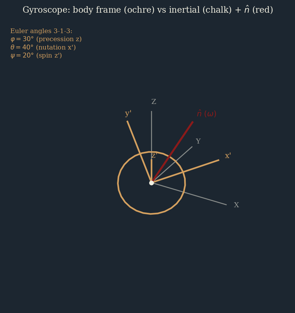
Fig 4.
The gyroscope’s three rotational degrees of freedom: φ (precession) about the vertical + θ (nutation) about the line of nodes + ψ (spin) about the body z axis. Euler’s rotation theorem tells us: even when the three angles change at the same time, at each instant the overall composition is still a pure rotation about
a unique instantaneous axis
.
Video correspondence
Video 11:16–14:51 (segment M3): - 11:16–11:45: Berlin Academy seal + Découverte 1750 + the first rigid-body equation (anim-26) - 11:45–12:20: rigid body vs fluid split-screen comparison (anim-27) - 12:20–12:55: switching body-fixed frame ↔ inertial frame (anim-10) - 12:55–13:30: gyro 3D + Euler angles φ/θ/ψ ⭐ (anim-11) - 13:30–14:00: rigid-body equation 3-step build (anim-12) - 14:00–14:30: Euler’s rotation theorem + visualization of the instantaneous axis (anim-13) - 14:30–14:51: 15-year arc 1750→1765 timeline (anim-14)
— Abel
§4 · Euler’s theorem and the RSA cryptosystem
Companion video: 14:53–15:55 (segment MISC_01)
This section assumes you are familiar with
: integer modular arithmetic (), the greatest common divisor , the extended Euclidean algorithm (finding modular inverses); introductory group theory (finite groups, Lagrange’s theorem) is optional — the main proof uses an elementary permutation and does not depend on group theory.
Historical note on notation
: Euler’s 1763 paper describes in Latin “the number of positive integers less than and coprime to ”, and
did not introduce the symbol
. The symbol in general use today comes from Gauss 1801
Disquisitiones Arithmeticae
§38 onward. This section uses for consistency with modern textbooks, but the reader should remember that Euler himself did not use this symbol.
Summary in one sentence
Euler’s theorem, published by Euler in 1763,
generalizes Fermat’s little theorem (when is prime, ) to an arbitrary positive integer modulus. More than two centuries later, in 1977, Rivest, Shamir and Adleman used this theorem to construct the RSA public-key cryptosystem — the first algorithm able to exchange keys securely over a public channel. This section gives the permutation proof of Euler’s theorem and a complete derivation of the correctness of RSA.
4.1 Definition and basic properties of the Euler function
Definition. For a positive integer , the Euler function is defined as the number of positive integers not exceeding that are coprime to :
Example: (note that all have a common factor with ).
Lemma A (prime case). If is prime, then (only itself is not coprime to ).
Lemma B (prime-power case). If is prime and , then .
Proof. In , those not coprime to are exactly the multiples of : , of them in all.
Lemma C (multiplicativity). If , then
Proof sketch. By the Chinese remainder theorem (CRT), modulo corresponds to modulo jointly:
The orders of the two sides are equal, which gives the conclusion.
Corollary (computational formula). If is the prime factorization of , then
4.2 The permutation proof of Euler’s theorem
Theorem (Euler 1763). If , then
Proof (using a multiplicative permutation).
Step 1. Let be the set of all elements of coprime to (that is, the representatives of ).
Step 2. Consider the set . We prove that this set equals the original set modulo (only in a different order, that is, a permutation).
- The elements are coprime to : since , we have (multiplicativity), so each belongs to .
- The elements are pairwise distinct: if with , then ; since , by the cancellation law , contradicting .
By these two points, is a permutation of .
Step 3 (the product is invariant). Multiply all the elements of the sets on both sides:
The left side rearranges to , so
Step 4 (cancel ). Since holds for each , , and a multiplicative inverse can be taken modulo . Multiplying both sides by gives
Concrete calculation (n=10, a=3).
- The coprime set .
- Multiply by : , exactly a permutation.
- Product: .
- Cancelling gives ; check: ✓.
🎬 n=10 permutation animation + derivation 3-step build — video 14:53 (anim-15): multiplied by lands on — visualization of the set mapping to itself + the abstract derivation, chunk MISC_01.
4.3 Fermat’s little theorem as a special case
Fermat’s little theorem (1640). If is prime and , then
As a special case of Euler’s theorem: take prime; Lemma A gives , and substituting into Euler’s theorem yields Fermat.
Equivalent form (for any , not necessarily coprime):
(When , that is , both sides are modulo , and it still holds.)
Historically, Fermat’s 1640 letter stated only the conclusion; the first complete proof was given by Euler in 1736 (by induction using the binomial theorem). Euler’s permutation proof then generalized it to arbitrary .
Worked example: Fermat’s little theorem + a prototype of the Miller-Rabin primality test
Example 1 (direct check). Take , :
Example 2 (use in primality testing). Given a large integer , decide whether is prime — naive trial division up to is too slow. Fermat test: choose a random and compute with fast modular exponentiation:
- If , then must be composite (because if were prime, Fermat’s little theorem would require ).
- If , then may be prime (this cannot be decided, because there exist “pseudoprimes” such as the Carmichael number that satisfy it for all coprime ).
The Miller-Rabin (1976) improvement: write ( odd), and check whether the sequence has a turning point at . This gets around the Carmichael trap. Miller-Rabin is the industrial standard by which all of today’s RSA libraries (OpenSSL / GMP / Python sympy.isprime) generate large primes.
What this tells us: Fermat’s little theorem is not merely a number-theory toy; it is the algorithmic core of primality testing in actual present-day engineering — when Euler generalized this theorem in 1763, he could not possibly have foreseen that 213 years later it would become the cryptographic foundation of internet security (TLS / SSH / PGP).
4.4 The RSA public-key cryptosystem
The core problem of RSA: how can encrypted information be transmitted over a public channel? The key observation is the difficulty of factoring large integers — even if the product of two large primes is known, when each have several hundred decimal digits, all existing algorithms need an infeasible amount of time to factor .
Step 1: key generation
- Choose two large primes (in practice each bits).
- Compute (the public modulus).
- Compute (by the multiplicativity Lemma C and the prime case, ).
- Choose satisfying and (the public encryption exponent; in practice is commonly taken).
- Compute satisfying — that is, , found with the extended Euclidean algorithm. is the private key (the decryption exponent).
Public key: , published openly. Private key: , kept strictly secret.
Step 2: encryption
For a plaintext , compute the ciphertext
Step 3: decryption
For a ciphertext , compute
Correctness theorem:
To prove:
Proof.
means that there exists a positive integer such that
Therefore
Case A: . By Euler’s theorem , so
Case B: . First exclude the boundary case (here , ✓, which obviously holds). Let , . Since is a product of two primes, we must have or (but not both, otherwise , that is , a contradiction). Without loss of generality let . Then
On the other hand , and by Fermat’s little theorem , so
By the Chinese remainder theorem (CRT): and jointly give
Where the security comes from
The security of RSA rests on the following computationally hard problem:
- Factoring large integers: since is public, if could be factored efficiently then could be recovered, from which could be computed, and then found — broken.
- The currently best factoring algorithm (the Number Field Sieve) has subexponential complexity , which is still infeasible for at the scale of bits — estimated to require a modern supercomputer running continuously for millions of years.
Note: if quantum computers are scaled up, Shor’s algorithm can factor large integers in polynomial time, and RSA will no longer be secure. This is the current core problem of post-quantum cryptography.
RSA Python toy trace (p=61, q=53)
Below, Python is used to walk through the three steps above, key generation / encryption / decryption. Although the toy parameters are small, every step is completely isomorphic to real-world 2048-bit RSA — only the numbers are 600 digits bigger.
from math import gcd

# --- Step 1: key generation ---
p, q = 61, 53                         # two (toy) primes
n = p * q                             # public modulus
phi = (p - 1) * (q - 1)               # Euler totient
print(f"n   = {n}")                   # 3233
print(f"φ(n)= {phi}")                 # 3120

e = 17                                # public encryption exponent, satisfies gcd(e, φ) = 1
assert gcd(e, phi) == 1

# find the modular inverse d ≡ e⁻¹ (mod φ), built into Python 3.8+:
d = pow(e, -1, phi)
print(f"e   = {e}, d = {d}")          # e=17, d=2753
assert (e * d) % phi == 1             # ed ≡ 1 (mod φ)  ✓

# --- Step 2: encryption ---
m = 65                                # plaintext (assumed already encoded as an integer < n)
c = pow(m, e, n)                      # ciphertext c = m^e mod n
print(f"plaintext m = {m}")           # 65
print(f"ciphertext c = {c}")          # 2790

# --- Step 3: decryption ---
m_prime = pow(c, d, n)                # m' = c^d mod n
print(f"decrypted m' = {m_prime}")    # 65
assert m_prime == m                   # correctness  ✓
Output of the run:
n   = 3233
φ(n)= 3120
e   = 17, d = 2753
plaintext m = 65
ciphertext c = 2790
decrypted m' = 65
Key observation: the person holding the private key can compute instantly; an attacker without the private key who wants to work back from to must first factor — with toy parameters this is solved in a second, but at the -bit scale (even with the most advanced NFS algorithm), the estimate exceeds the lifetime of a modern supercomputer. This is the core of asymmetric encryption: encryption / verification use the public key, decryption / signing use the private key, and the two are strung together on one thread by Euler’s theorem.
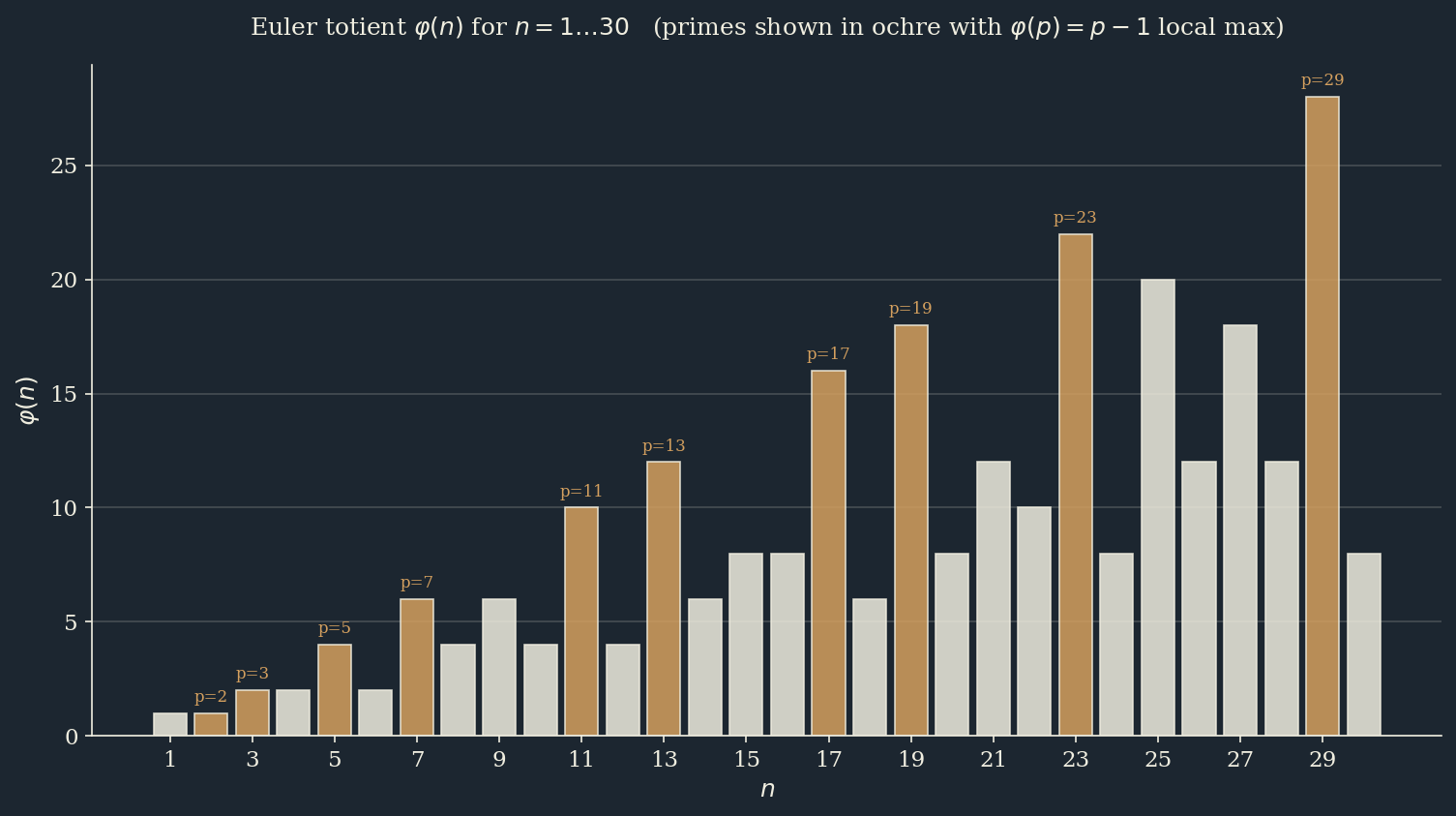
Fig 5.
Values of the Euler totient for . Orange = at primes, , a local maximum; blue = at composites, where drops markedly, reflecting that composites have more small elements not coprime to them. This jagged shape is exactly one of the sources of RSA’s security: even knowing , is hard to predict directly; one must first factor.
Geometric/physical intuition
The geometric flavor of Euler’s theorem is hidden in group theory. is a finite commutative group of order . For any element of the group, by Lagrange’s theorem, the order of (that is, in , the smallest positive integer ) must divide the order of the group , and hence — this is the group-theoretic reading of Euler’s theorem.
More intuitively, our earlier permutation proof showed: multiplying by each element of amounts to performing a permutation on that finite set — the elements are shuffled, but the set itself is unchanged. In any finite group the operation “multiply by ” is a permutation, and this fact directly gives Lagrange’s theorem and Euler’s theorem.
And the core magic trick of RSA lies in:
If encryption is regarded as turning the message around the finite wheel by turns, decryption is turning it back by turns; and guarantees exactly that the total number of turns equals ” turn plus an integer multiple of turns” — by Euler’s theorem, turns equals not turning at all — so it finally returns to the starting point.
Video correspondence
Video 14:53–15:55 (segment MISC_01): - 14:53–15:18: demonstration of the permutation of the coprime set multiplied by (anim-15 Phase 1-4) - 15:18–15:55: the abstract derivation in three steps (anim-15 Phase 5)
Suggested further reading: - Koblitz, A Course in Number Theory and Cryptography (Springer GTM 114) - RFC 8017: PKCS#1 v2.2 (RSA implementation standard)
— Abel