The Nobel Prize in Physics (1) 1901: Röntgen, and an Invisible Light

Companion video (YouTube): original English narration, switchable Chinese dubbing, Chinese and English subtitles

The starting point of this series is a teacher of mine. He is always willing to share something with everyone on WeChat Moments.

I am not an expert, nor a professor, just a person who likes science. In the age of artificial intelligence I often feel lost, but I have not given up the things I love.

This series is dedicated to people who are just as lost: to those who dare to face the unknown, to those who walk into the unknown to explore it, and also to those who have never stopped, who keep walking toward their dreams.

And let us also not forget those pioneers.

In November 1895, in the Physical Institute of the University of Würzburg, a paper screen lit up by itself in the dark. This episode first tells what Röntgen saw, what kind of person he was, and how the news spread, then how it is explained today, and finally the prize six years later, and the dispute around this discovery.

Winter 1895, Würzburg

The official Nobel Prize biography of Röntgen says that on the evening of November 8, 1895, Wilhelm Conrad Röntgen was working with a discharge tube in the Physical Institute of the University of Würzburg. Many people were using tubes of this kind at the time: a glass tube is pumped down to a near vacuum, a high voltage is applied across its two ends, and something called cathode rays appears inside the tube, striking the glass wall and making it fluoresce. Röntgen had wrapped the tube tightly in thin black cardboard, so by rights no light at all should have got through, yet a paper screen nearby, coated with barium platinocyanide, lit up, and it still lit up when moved two meters away.

Over the next few weeks he did a large number of experiments, alone. Paper, a thick book of a thousand pages, wooden boards two or three centimeters thick could not stop it; thin metal sheets let it through too, the thicker and heavier the metal, the more it stopped, and lead one and a half millimeters thick let almost nothing through. On December 28 he submitted a paper as a manuscript to the Würzburg Physical-Medical Society, titled “On a New Kind of Rays (Preliminary Communication)” (Ueber eine neue Art von Strahlen, Vorläufige Mittheilung). In Section 2 of the paper there is a sentence saying that if you hold your hand between the discharge tube and the fluorescent screen, you can see the darker shadows of the hand bones, surrounded by the fainter outline of the hand. On the same page there is a footnote in which he says that, for brevity, and to distinguish them from other rays, he will call them “X-rays” for the time being.

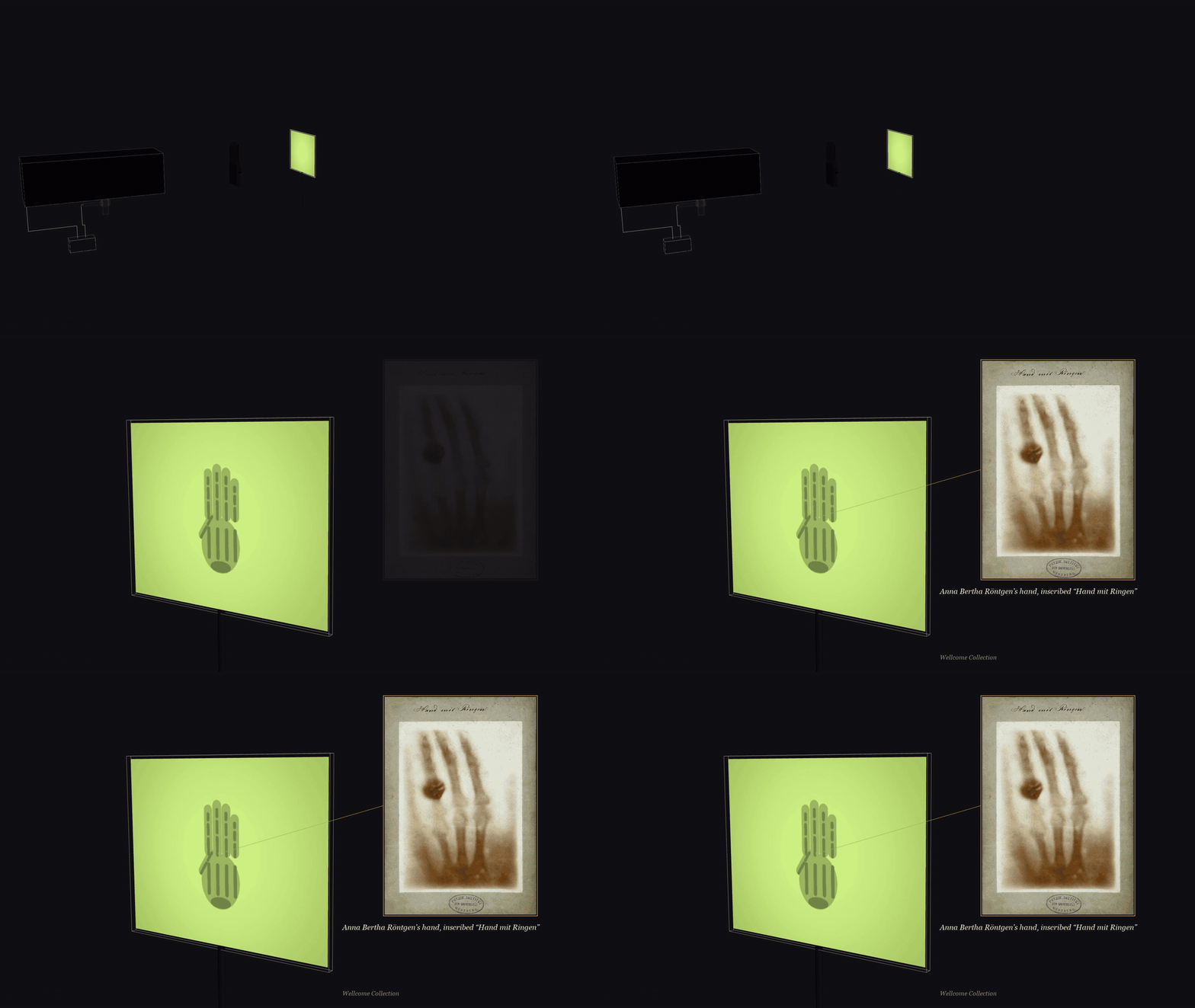
A hand between the tube and the screen casts the shadow of its bones; on the right, the 'hand with rings' print Röntgen sent to colleagues.

Figure 1. A hand between the tube and the screen casts the shadow of its bones; on the right, the ‘hand with rings’ print Röntgen sent to colleagues.

This paper had not a single illustration. The hand bones appeared only in the text.

The photograph of hand bones that everyone has seen today, with a ring on a finger, shows the hand of his wife, Anna Bertha Röntgen. Several museums catalogue its date as December 22, 1895, but at present no primary evidence can be found to prove this date; the original photograph bears only the words “hand with ring, §2 and §14” (translated), referring to two sections of the paper. Nor has any museum catalogued a negative from this exposure. What survives are a few paper prints Röntgen made himself, which around New Year 1896 he sent to several colleagues together with offprints of the paper, and which are now held separately at the German Röntgen Museum, the Wellcome Collection in London, the Teylers Museum in the Netherlands and elsewhere. As for the line she said when she saw the photograph, “I have seen my own death” (translated), the earliest direct quotation we found is a 2010 blog post that gives no source; earlier printed material has not been fully searched. Röntgen’s biographer Otto Glasser, in his 1945 book, writes only that when she thought that what she was looking at was a skeleton, she shuddered.

The earliest printing that can be found at present is in the British journal Nature of January 23, 1896, where the caption says: the bones of the fingers of a living person, with a ring on the third finger. The caption does not say whose hand it is, but judging from the cropping, it is this one.

On the same day, Röntgen gave a lecture at the Würzburg Physical-Medical Society. The Society’s minutes record the scene: on the spot, he took an image of the bones of the right hand of the Society’s honorary president, the anatomist Albert von Kölliker. Kölliker then proposed that the new rays be called “Röntgen rays”, and the whole hall cheered.

Röntgen the man

Before talking about this light, let us first lay out his life roughly in order. Each entry is followed by its sources; where several accounts do not agree, we write all of them down.

March 27, 1845 Born in Lennep in the Prussian Rhine Province (now part of Remscheid), the only child of the family. His father was a cloth merchant who also ran a woolen-cloth factory; his mother came from Amsterdam. [Official Nobel Prize biography; Neue Deutsche Biographie]
1848 The family moved to Apeldoorn in the Netherlands, where he went to a local boarding school. [Official biography; Neue Deutsche Biographie]
1862 Entered a technical school in Utrecht (the University of Würzburg Archives give 1861), and left without obtaining a diploma. The official biography says that he was expelled after being wrongly accused of drawing a caricature of a teacher; the University of Utrecht’s account is that he did not pass the final examination; a historian of science at the University of Munich wrote in 2023 that the caricature story has no evidence behind it. The year he left the school is also given differently by different sources, some 1863, some 1864. [Official biography; University of Utrecht; Neue Deutsche Biographie; University of Würzburg Archives; University of Munich 2023]
1865 Early in the year, an auditing student at the University of Utrecht, not allowed to take examinations; that winter, entered the Federal Polytechnic School in Zurich (today’s ETH) to study mechanical engineering. [University of Utrecht; University of Zurich]
1868 Received his diploma as a mechanical engineer. While studying in Zurich, he attended lectures by Rudolf Clausius and also entered the laboratory of August Kundt. [Official biography; Neue Deutsche Biographie; University of Zurich; Glasser]
1869 Received his doctorate from the University of Zurich with a thesis on gases (Neue Deutsche Biographie gives 1870). After that he became Kundt’s assistant, and in 1870 followed him to Würzburg. [University of Zurich; University of Würzburg Archives; Glasser]
1872 On January 19, married Anna Bertha Ludwig in Apeldoorn; in April, followed Kundt again, to the newly founded University of Strasbourg. [Apeldoorn marriage register, 1872 (archive index); Neue Deutsche Biographie; Glasser]
1874–1879 In 1874 obtained his habilitation in Strasbourg (Neue Deutsche Biographie gives 1873); in 1875 became professor of physics and mathematics at the Hohenheim Agricultural Academy; in 1876 returned to Strasbourg as associate professor of physics; in 1879 became full professor of physics at the University of Giessen. [Official biography; Neue Deutsche Biographie; Glasser]
1888 Became professor of physics at the University of Würzburg and director of its Physical Institute; in 1893 or 1894 was elected rector (the University of Würzburg Archives give 1893, Glasser gives 1894). What happened on the evening of November 8, 1895, happened in this Physical Institute. [Neue Deutsche Biographie; University of Würzburg Archives; Glasser]
1900 At the request of the Bavarian government, went to the University of Munich as professor of experimental physics and director of its Physical Institute. [Neue Deutsche Biographie; University of Munich; official biography]
December 10, 1901 Received the first Nobel Prize in Physics in Stockholm. [Official Nobel Prize]
1919–1923 His wife died in 1919; he retired in the spring of 1920; he died in Munich on February 10, 1923. In accordance with his wishes, his ashes were buried together with his parents and his wife in the Old Cemetery in Giessen. [Official biography; Neue Deutsche Biographie; University of Giessen; obituary, reproduced in facsimile in Glasser’s book]

How the news spread

After the paper was handed in, the news spread extremely fast. On January 5, 1896, the Vienna newspaper Die Presse ran “A sensational discovery” on its front page, and the paper printed Röntgen’s name as Routgen.

The doctors were the most eager. On January 24, the Viennese surgeon von Mosetig-Moorhof reported two cases at the Society of Physicians in Vienna; in one of them, the patient had a 6-millimeter lead bullet in the palm of his left hand, and its position had been found with a Röntgen photograph.

In Montreal, Canada, a man was shot in the leg on the evening of Christmas Day 1895. On February 7, 1896, the physicist Cox exposed his leg for 45 minutes, and on the plate the flattened bullet was lodged between the tibia and the fibula. The next day the surgeon Kirkpatrick operated and took the bullet out. In May of the same year, an editorial in the Montreal Medical Journal wrote that this was “one of the first cases” in which this new kind of photograph was taken into court as evidence; the man who fired the shot was sentenced to fourteen years.

That year, X-rays became the talk of the town. New York’s Life magazine published a cartoon titled “The New Roentgen Photography. ‘Look pleasant, please.’”, and what the photographic plate shows is a skeleton holding a scythe. In February, the New Jersey legislator Reed introduced a bill in the state legislature to prohibit the use in theaters of opera glasses made with X-rays or cathode rays; the Speaker ruled the bill out of order.

In the bibliography Otto Glasser compiled in 1931, for the single year 1896 alone, 49 books and pamphlets on X-rays are listed, and nearly a thousand journal articles.

In May, at the National Electrical Exposition in New York, Edison set up an X-ray stand; visitors went in two at a time, lining up to look at the bones of their own hands on a fluorescent screen. According to the report in the Electrical Review, the machine was operated by several assistants from Edison’s laboratory: Fred Ott, Charles Brown and Clarence Dally.

But very soon people found that these rays were not harmless. In February of that year, the physics laboratory of Vanderbilt University in the United States received a request to locate a bullet in the head of a child who had been accidentally shot. On February 29, John Daniel and Dr. William L. Dudley decided to try it out first: Dudley used his own head as the test subject, with the tube about half an inch from his hair, and exposed it for one hour. On March 23, Daniel wrote to the journal Science: nothing at all came out on the plate, but on the 21st day after the test, all the hair fell out of the patch that had been exposed.

Dally later did X-ray experiments for many years, and his fingers and both arms were amputated, piece by piece. In August 1903, the New York Times reported that Edison’s eyes had also been injured by the rays in experiments more than two years earlier; in the same month, “Don’t talk to me about X rays,” he said to a reporter, “I am afraid of them.” On October 2, 1904, Dally died, and the New York Times headline called it a martyrdom for science.

The development of science is sometimes not entirely harmless. Those who pay the price first are often the people closest to it.

What kind of light was it

Röntgen himself did not know. The presentation speech of 1901 also said so very honestly: what exactly this radiation is, is not yet clear.

Today’s answer is this. The high voltage across the two ends of the tube accelerates electrons, and the electrons, carrying kinetic energy, hit the glass wall. The vast majority of the energy turns into heat, but a small part is light emitted when an electron is violently pulled off course and slowed down near an atomic nucleus. This light is called Bremsstrahlung, which in German means “braking radiation”. Electrons are braked some lightly and some heavily, so the light they emit has energies some high and some low, and therefore the X-ray spectrum is one continuous band.

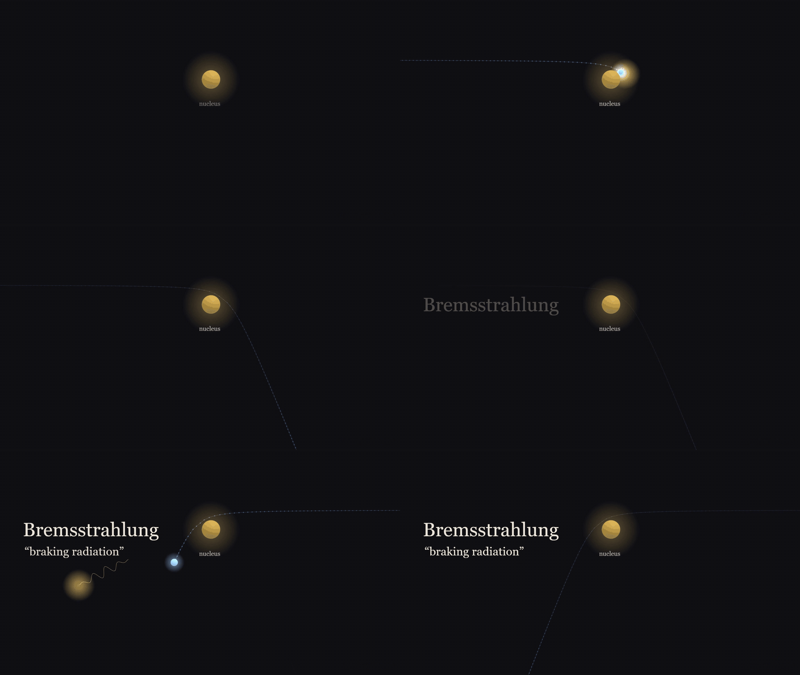
An electron swerves and slows near a nucleus and gives off a photon: bremsstrahlung, braking radiation.

Figure 2. An electron swerves and slows near a nucleus and gives off a photon: bremsstrahlung, braking radiation.

This continuous spectrum has one very strange feature: it has a sharp upper limit (when the voltage fluctuates, the limit is set by its highest moment). If the accelerating voltage is V, the electron’s kinetic energy is at most eV, and the energy of the emitted light is also at most eV, with nothing at all above it. In terms of wavelength, there is a shortest wavelength λ_min = hc/eV. For example, at a voltage of 30 kilovolts the shortest wavelength is 0.041 nanometers; raise the voltage to 100 kilovolts and the shortest wavelength shrinks to 0.012 nanometers. According to classical electromagnetism, an accelerated charge should radiate a smooth spectrum, with no such hard edge: conservation of energy governs only the total energy radiated, not the frequency, and any frequency can carry away just a tiny bit of energy. What this edge says is that energy is exchanged in portions: light of frequency ν must take away at least hν of energy each time, and an electron has at most eV to give, so the frequency is capped. This was only understood later. As for whether light itself is made of individual particles, this edge alone cannot show that. The view that light consists of photons became generally accepted only after Compton scattering, which we leave for that episode.

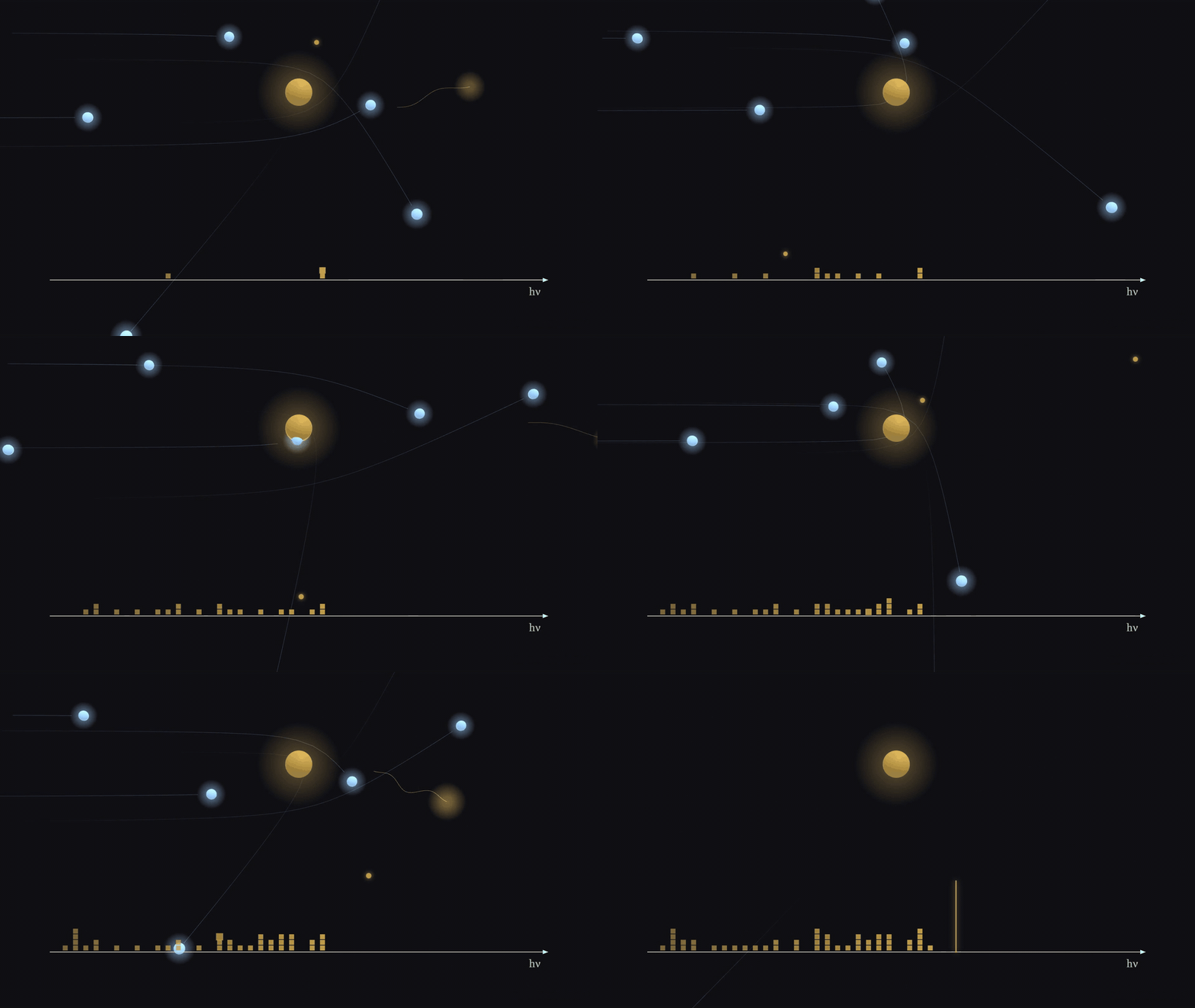
Some electrons brake hard, some gently, so the photons pile up into a continuous spectrum, with a sharp edge at eV.

Figure 3. Some electrons brake hard, some gently, so the photons pile up into a continuous spectrum, with a sharp edge at eV.

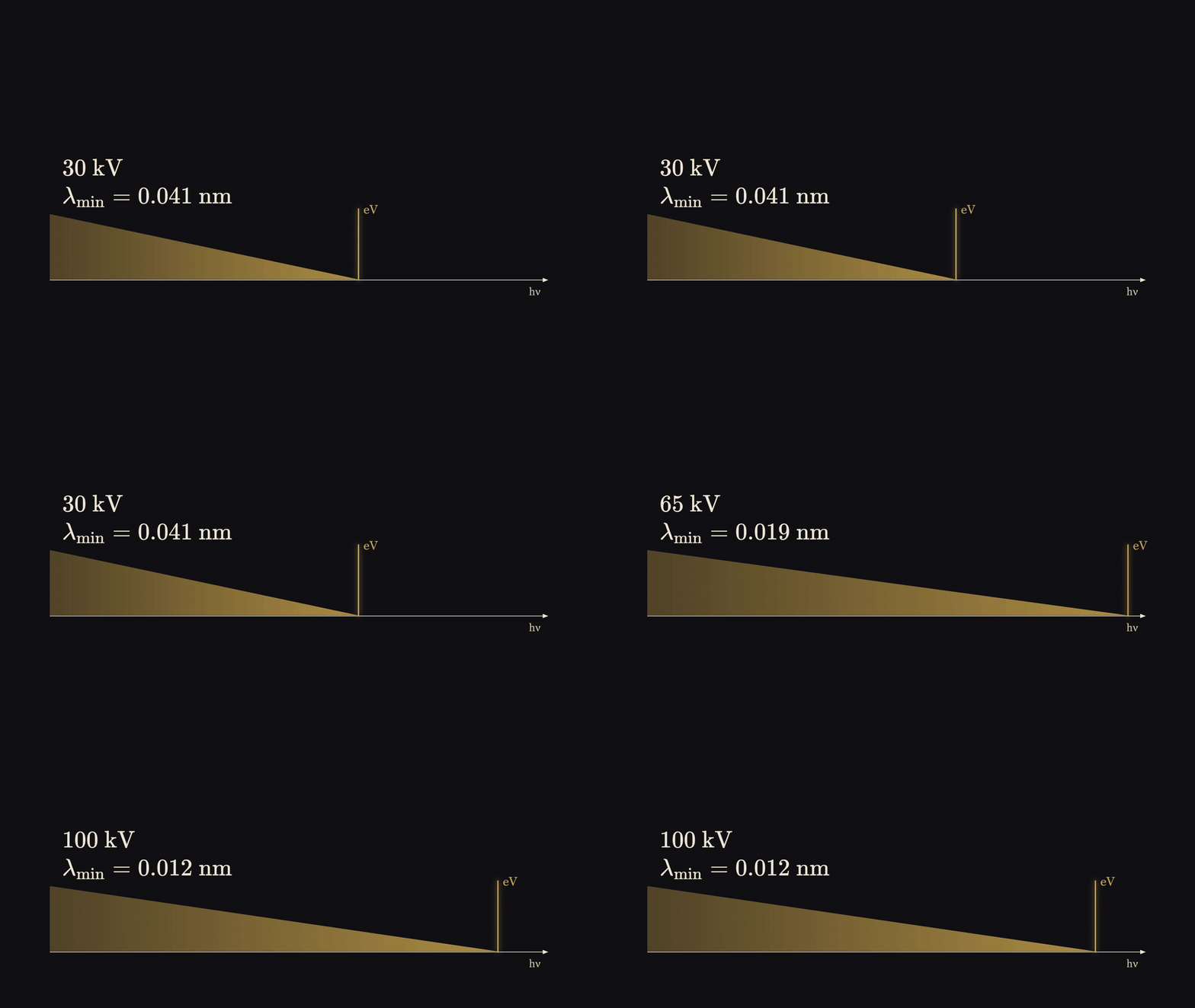
Raising the voltage from 30 to 100 kV moves the shortest wavelength from 0.041 to 0.012 nm.

Figure 4. Raising the voltage from 30 to 100 kV moves the shortest wavelength from 0.041 to 0.012 nm.

There is one more detail to make clear. Röntgen used a cold-cathode discharge tube, and there was no metal target in the tube. In Section 12 of his paper he wrote that the X-rays are emitted from the spot where the cathode rays hit the glass wall, and when he used a magnet to move the cathode rays aside, the point of emission moved with them. Only a few months later, in early 1896, did he switch to a platinum plate as a target. The hot-filament, tungsten-target X-ray tubes in today’s hospitals are a later thing. What glass his tube was made of, the paper does not say; according to secondhand accounts from collectors, tubes of this kind were generally soda-lime glass. Light elements such as silicon, oxygen, sodium and calcium all have very low characteristic line energies, which are absorbed by the tube wall, so as long as the glass contains no heavy element such as lead, what Röntgen saw was essentially all braking radiation.

Why bones show up

When monoenergetic X-rays pass through a layer of something, the intensity decays exponentially: each equally thin layer passed through takes away the same proportion. How fast or slow the attenuation is depends on the material itself. Why bone is darker than flesh: the common explanation is that bone is denser. That is only half right.

Computing with the standard data tables of the US National Institute of Standards and Technology (NIST), taking the density of cortical bone as 1.92 grams per cubic centimeter and soft tissue as 1.06: at a photon energy of 20 kiloelectronvolts, the attenuation coefficient of bone is 8.8 times that of flesh: 1 centimeter of flesh lets through 42%, 1 centimeter of bone only 0.05%. When the energy rises to 100 kiloelectronvolts, this factor drops to 2.0; at 1 megaelectronvolt, only 1.70 is left.

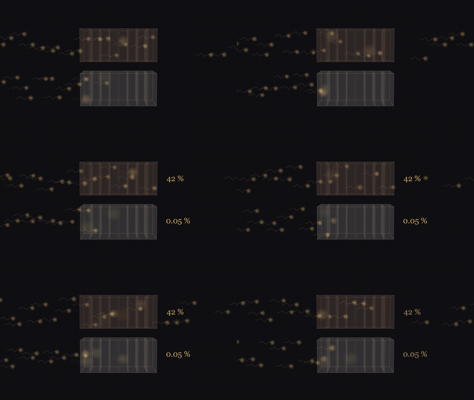
One centimetre at 20 keV: 42% gets through soft tissue, 0.05% through bone.

Figure 5. One centimetre at 20 keV: 42% gets through soft tissue, 0.05% through bone.

The number 1.70 is almost exactly the product of two things: the density ratio of bone to flesh, 1.81, times the ratio of the number of electrons per gram of material, 0.936, which gives 1.69. At very high energies, X-rays are mainly scattered away by electrons, and they recognize only how many electrons there are, so at that point only one cause is left: the number of electrons per unit volume. Bone is denser, but per gram it actually has slightly fewer electrons, and multiplying these two gives the number above. At low energies the ratio is much larger, more than 5 times the high-energy value at 20 kiloelectronvolts, and the extra part comes almost entirely from another process: the photoelectric effect. The photoelectric effect is extremely sensitive to atomic number; bone contains calcium and phosphorus, with atomic numbers 20 and 15, while flesh is mainly carbon, oxygen and hydrogen. So bone is dark for two reasons, one is that it is dense, the other is that its atomic number is high, and the second reason gradually disappears as the energy rises.

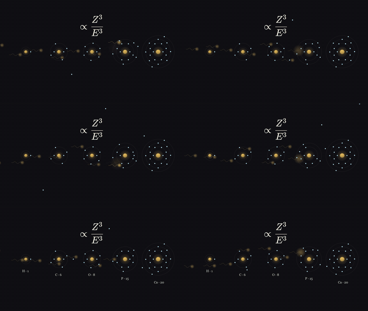
The photoelectric effect grows roughly as the cube of the atomic number: H, C, O, P, Ca, each absorbs more than the last.

Figure 6. The photoelectric effect grows roughly as the cube of the atomic number: H, C, O, P, Ca, each absorbs more than the last.

The derivations for this section, including the attenuation formula and how these numbers were obtained, are in Appendix A.

December 1901, Stockholm

On December 10, 1901, in the hall of the Royal Academy of Music in Stockholm, the Nobel Prizes were awarded for the first time. The Physics Prize went to only one person, Röntgen, and the citation was: in recognition of the extraordinary contribution he made by discovering the remarkable rays later named after him.

King Oscar was not there that day, and the prizes were presented on his behalf by Crown Prince Gustaf. A twenty-year-old student who served as a marshal at the time later recalled that the first to enter was that “stately German” (translated), with a large dark professor’s beard. Röntgen in fact did not much want to come. In his letter requesting leave to the Bavarian Ministry of Culture and Education, he wrote that the Academy placed special importance on the prizewinners appearing in person, and that although he was reluctant, he also felt he ought to comply, so he was requesting a week’s leave. He came, received the diploma and the medal, but did not give a Nobel lecture. The official lecture page to this day has only one sentence: “No Lecture was delivered by Professor W. Röntgen.”

The dispute: Lenard

The nomination archive for 1901 was opened fifty years later. That year the Physics Prize received 29 valid nominations in all, 16 of them for Röntgen, including one from Max Planck. One is quite interesting: Röntgen himself nominated Lord Kelvin.

Of these 16, 5 are worth looking at separately. The newly established Nobel Committee for Physics had five members in all, and all five of them nominated the same pairing: Philipp Lenard and Röntgen jointly. The plenary session of the Academy finally decided to give the prize to Röntgen alone. Whom the committee itself later recommended to the Academy, and on what grounds: the committee’s report is not on the public archive web pages, and we have not seen it.

Lenard worked on cathode rays. He had made a kind of discharge tube with an extremely thin aluminum-foil “window” in the tube wall, which let cathode rays escape outside the tube. Röntgen’s first paper mentions him five times: at the beginning, when listing the tubes that can be used, it mentions “Lenard-type” ones (translated), and Section 10 specifically mentions Lenard’s experiments in which cathode rays passed through thin aluminum sheets. According to the Dictionary of Scientific Biography (secondary), Lenard gave Röntgen a tube at Röntgen’s request. But the paper does not say which tube he actually used that day in November.

Four years later, the 1905 Physics Prize went to Lenard, for his work on cathode rays. In May 1906 he gave his Nobel lecture in Stockholm, and he mentioned Röntgen in only one place. He said that Röntgen was the first to use the kind of tube he had described, and that the discovery of X-rays is usually regarded as a lucky discovery, but in his view, once there was that kind of tube, the observer’s attention had already shifted from inside the tube to the outside, and a fluorescent screen was in any case already placed outside the tube, so at that stage the discovery was bound to be made sooner or later.

Later he put it more and more strongly. In 1929 he wrote to Röntgen’s biographer that there was no doubt the road to this discovery had passed over his research. By 1945, he was telling people that he was the mother of X-rays; that just as a midwife need not be responsible for the mechanism of birth, Röntgen need not be responsible for the discovery of X-rays; it had simply fallen into his lap. We have seen these two statements only as quoted by the biographer; we have seen neither the original letter nor any record of the conversation. In the 1930s Lenard became the standard-bearer of the Nazi “German Physics”, and according to Glasser, in the four-volume physics textbook Lenard wrote, the main text mentions neither Röntgen nor Einstein.

To the things Lenard said while Röntgen was alive, including the 1906 lecture, Röntgen never responded publicly, at least nothing is recorded in the sources we found; when the two statements of 1929 and 1945 were made, Röntgen had already died, in 1923. In his will he asked that all the papers in the cupboard in the hallway of his Munich apartment be burned, and the executor said that the letters from the period of the discovery were all burned. So how he thought about this dispute, we cannot find any record he left himself.

Prize money and patents

Many places online write that Röntgen’s prize money was 50,000 Swedish kronor, and that he donated it to the University of Würzburg. In the Nobel Foundation’s table of prize amounts, the 1901 Physics Prize was 150,782 kronor. In 2023 someone read all of Röntgen’s will documents in the Bavarian State Archives: his 1911 will left 200,000 marks to a physics research foundation for pure science, and in 1920 this was changed to the Physical Institute of the University of Würzburg. The amount of this money is about the same as the prize money, but the will does not mention the Nobel Prize by a single word. The inflation after the First World War then swallowed up almost all of these bequests. So all that can be said is: he left a sum of money comparable to the prize money to the Physical Institute of the University of Würzburg. “Donated his Nobel Prize money” is the biographers’ interpretation.

He never applied for a patent on X-rays; all accounts agree on this, but they are all secondhand. As early as January 1896, a London company wrote to him proposing commercial development. The often-quoted line “inventions and discoveries belong to the whole world” (translated) can at present be found only in secondhand sources.

Afterwards

In that 1895 paper Röntgen tried to make X-rays refract and to make them reflect regularly, and measured neither, but he did find that plates of platinum, lead and zinc reflected them back diffusely. At the end of the paper he says that these rays are completely different from the known infrared, visible light and ultraviolet, and guesses that they might be longitudinal waves in the ether. It was not that he did not dare to say it was light; it was that he would not say it was a known kind of light.

This question dragged on for a long time. In 1912, Walter Friedrich and Paul Knipping, following a suggestion by Max von Laue, sent X-rays through a crystal and photographed diffraction spots, showing that they are waves; in 1915, William Duane and Franklin Hunt precisely measured that cutoff edge in the spectrum, and that edge in turn pointed to quanta. Laue, the Braggs (father and son), Barkla, Siegbahn and Compton later all received the Physics Prize for work related to X-rays; we will talk about them when we reach those years.

The next episode is 1902, Hendrik Lorentz and Pieter Zeeman: put a light source into a magnetic field, and the spectral lines broaden.

Appendix A: Physics derivations

The two sections in the main text, “What kind of light was it” and “Why bones show up”, covered only the concepts. This appendix derives them from the beginning, and each result is followed by an example you can compute yourself. The data are taken from several public databases of the US National Institute of Standards and Technology (NIST). One point must be made first: NIST’s attenuation coefficient tables are compiled from theoretically calculated atomic cross sections, not measured directly on bone and flesh; the values for compounds and mixtures are calculated from the elements by weighting, according to the mixture rule in Section A.3 below.

Notation in this appendix

Symbol	Meaning
$e$	magnitude of the electron charge, $1.602176634\times10^{-19}$ coulomb
$V$	accelerating voltage across the tube
$K$	kinetic energy of the electron
$m_e$	electron mass, $m_ec^2 = 510.999$ keV
$h$ , $\hbar$	Planck constant, $\hbar = h/2\pi$
$c$	speed of light
$\nu$ , $\lambda$	frequency and wavelength of light, $\lambda\nu = c$
$\alpha$	fine-structure constant, $\alpha = e^2/(4\pi\varepsilon_0\hbar c) \approx 1/137$
$\mu$	linear attenuation coefficient, in cm $^{-1}$
$\rho$	density, in g/cm $^3$
$\mu/\rho$	mass attenuation coefficient, in cm $^2$ /g
$\sigma$	cross section, in cm $^2$ or barns (1 b $=10^{-24}$ cm $^2$ )
$N_A$	Avogadro constant
$Z_i$ , $A_i$	atomic number and molar mass (g/mol) of the $i$ -th element
$w_i$	mass fraction of the $i$ -th element in a mixture
$\langle Z/A\rangle$	the mixture’s average $\sum_i w_iZ_i/A_i$

A.1 Energy in the tube

Definition A1.1 (electronvolt). The work done by the electric field on an electron passing through a potential difference of 1 volt is called 1 electronvolt, written eV:

1\ \text{eV} = 1.602176634\times10^{-19}\ \text{J}. \tag{A1.1}

A kiloelectronvolt is written keV, a megaelectronvolt MeV.

The thing the electron finally hits is called the target. In Röntgen’s tube, the target was the patch of glass wall struck by the cathode rays; in later X-ray tubes, the target is a piece of metal placed there specially.

Proposition A1.1. An electron that starts near the cathode with negligible initial velocity and passes through a potential difference $V$ to hit the target has, on arrival, kinetic energy satisfying $K \le eV$ . If the target is at the anode potential and the electron collides with nothing on the way, equality holds.

Proof. The electrostatic field is conservative: when a charge $q$ goes from potential $\varphi_1$ to $\varphi_2$ , the work done by the electric force is $q(\varphi_1-\varphi_2)$ , independent of the path taken. The electron carries charge $-e$ ; going from the cathode to the target, at a potential $V'$ higher, the electric force does work $eV'$ , and $V'$ does not exceed the voltage $V$ between cathode and anode. By the work–energy theorem, the increase in kinetic energy equals the work done by the net force; if it collides with gas molecules on the way, it loses additional energy, so $K \le eV' \le eV$ . When the target is at the anode potential, $V' = V$ , and with no collisions, $K = eV$ . (QED)

Example A1.2. At a voltage of 30 kilovolts, the electron hits the target with a kinetic energy of at most $K = 30$ keV $= 4.807\times10^{-15}$ J. At this point the electron is already fast enough that relativity has to be considered. Kinetic energy and speed are related by $K = (\gamma-1)m_ec^2$ , $\gamma = 1/\sqrt{1-v^2/c^2}$ . Substituting gives $\gamma = 1 + 30/511 = 1.0587$ , $v/c = 0.328$ , $v = 9.84\times10^{7}$ m/s, about one third of the speed of light. Using Newtonian mechanics’ $K = \tfrac12 m_ev^2$ would give $v/c = 0.343$ , 4.4% too high; when the voltage rises to 100 kilovolts, the discrepancy grows to 14%.

Remark A1.3. Proposition A1.1 gives only an upper limit. Röntgen’s tube was filled with a rarefied gas, and the glass wall, once struck by electrons, becomes negatively charged itself; its potential is uncertain, and the electrons do not all get the full $eV$ . The cutoff wavelength in Section A.2 below uses only this upper limit.

A.2 Braking radiation and the cutoff wavelength

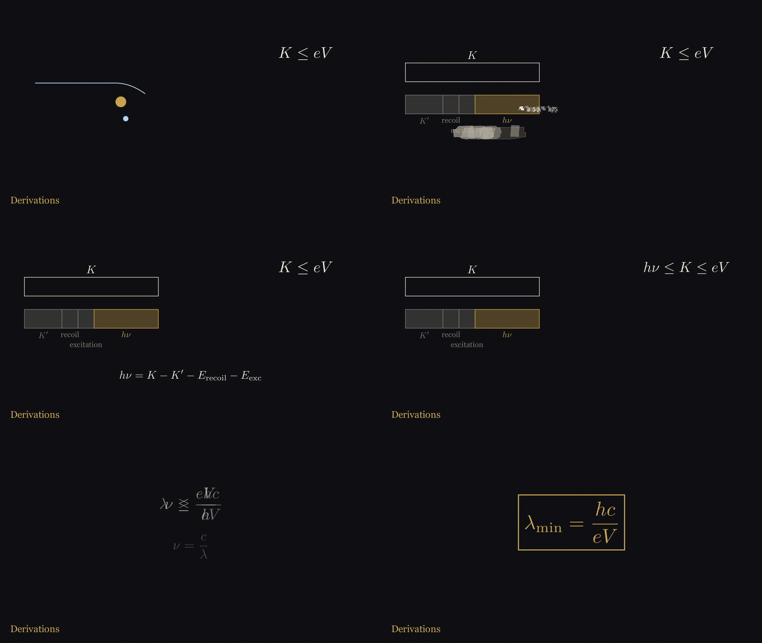
From 'the photon cannot carry more than the electron's kinetic energy' to λ_min = hc/eV, step by step.

Figure 7. From ‘the photon cannot carry more than the electron’s kinetic energy’ to λ_min = hc/eV, step by step.

Cited result A2.1 (Larmor formula). When a charge $q$ moves with acceleration $a$ at a speed much less than the speed of light, the total power it radiates in all directions is

P = \frac{q^2a^2}{6\pi\varepsilon_0c^3}. \tag{A2.1}

It is not derived here; for the derivation see Feynman, The Feynman Lectures on Physics, Volume I, Chapter 32, Eq. (32.5). Only one point matters: a charge moving at constant velocity does not radiate, and the strength of the radiation is proportional to the square of the acceleration. When an electron passes close by an atomic nucleus, it is violently pulled off course and slowed down by the Coulomb force; the acceleration is extremely large, and it emits light. This light is called Bremsstrahlung, whose original meaning in German is “braking radiation”.

Definition A2.2 (photon). Light of frequency $\nu$ can exchange energy only in portions; each portion is called a photon, and its energy is

E = h\nu = \frac{hc}{\lambda}, \qquad hc = 1239.842\ \text{eV·nm}. \tag{A2.2}

Proposition A2.3 (cutoff wavelength). Assume that each photon is emitted by one electron in one interaction. When the accelerating voltage is $V$ , in the X-ray spectrum emitted by the tube the photon energy does not exceed $eV$ ; in terms of frequency and wavelength, this is

\nu \le \nu_{\max} = \frac{eV}{h}, \qquad \lambda \ge \lambda_{\min} = \frac{hc}{eV}. \tag{A2.3}

Proof. Let the electron’s kinetic energy be $K$ before the interaction and $K' \ge 0$ after, and let the nucleus recoil with kinetic energy $K_N \ge 0$ ; if the atom is excited, an excitation energy $\Delta \ge 0$ is also taken away. By conservation of energy, $h\nu = K - K' - K_N - \Delta \le K$ . Then by Proposition A1.1, $K \le eV$ , so $h\nu \le eV$ . Substituting (A2.2) gives (A2.3). (QED)

Substituting the value of $hc$ , (A2.3) can be written in a handy form:

\lambda_{\min}\,[\text{nm}] = \frac{1.23984}{V\,[\text{kV}]}. \tag{A2.4}

Example A2.4.

Voltage	$\lambda_{\min}$	$\nu_{\max}$
30 kV	0.0413 nm	$7.25\times10^{18}$ Hz
50 kV	0.0248 nm	$1.21\times10^{19}$ Hz
100 kV	0.0124 nm	$2.42\times10^{19}$ Hz

The wavelength of visible light is between 400 and 700 nanometers. Compared with the shortest wavelengths in the table above, visible light is ten thousand to more than fifty thousand times longer.

Remark A2.5 (why this edge is called evidence of quanta). The proof of Proposition A2.3 used two premises: one photon is emitted by one electron, and the energy of light is given out in portions of $h\nu$ . Remove the second, and treat both the electron and the light by classical physics: conservation of energy still holds, but what it governs is the total energy radiated, not the frequency: a classical electromagnetic wave can carry just a tiny bit of energy at any frequency, so however high the frequency, it does not violate conservation of energy, and no edge determined by the electron’s energy appears in the spectrum for that reason. With the $h\nu$ premise, light of frequency $\nu$ must carry away at least $h\nu$ of energy, and only then does conservation of energy for the first time constrain the frequency, with the limit falling at $eV/h$ .

There is also a third treatment, called the semiclassical treatment: the electron’s energy changes according to quantum mechanics, while light is still treated as a classical wave. Then the electron jumps from a state with kinetic energy $K$ to a state with kinetic energy $K'$ , and the frequency of the emitted wave is fixed by Bohr’s frequency condition, $\nu = (K-K')/h$ . $K'$ cannot be less than 0, so again one gets $h\nu \le K$ , and again there is this edge, without photons being used anywhere. So what this edge proves is that energy is exchanged between electrons and light in units of $h\nu$ ; this is evidence of quanta. This edge alone cannot tell whether what is quantized is light itself, or only the electron’s energy.

In 1915 William Duane and Franklin Hunt precisely measured this edge: it is proportional to the voltage, and the proportionality constant is $e/h$ ; conversely, by measuring the voltage and the cutoff wavelength, one can compute the Planck constant. The view that light itself consists of individual photons became generally accepted in the physics community only after Compton scattering in 1923, which we leave for the episode on Compton’s prize.

Example A2.6 (how close it has to come to emit a 30 keV photon). A collision lasting a time $\tau$ emits light whose frequency reaches at most the order of $1/\tau$ . To emit a photon with an energy of 30 keV, the frequency is $\nu = 7.25\times10^{18}$ Hz, so the collision time cannot be longer than $1/\nu = 1.4\times10^{-19}$ s. An electron moving at $9.84\times10^7$ m/s travels only 14 picometers in this time (1 picometer $=10^{-12}$ meter), while the size of an atom is about 100 picometers. So high-energy photons come mainly from electrons that brush past very close to a nucleus. Electrons that enter the target hand over the vast majority of their energy bit by bit, in collision after collision with the electrons in the atoms, and it ends up as heat. This is only an order-of-magnitude estimate; the exact shape of the spectrum has to be computed with quantum mechanics.

A.3 Attenuation: the Beer–Lambert law

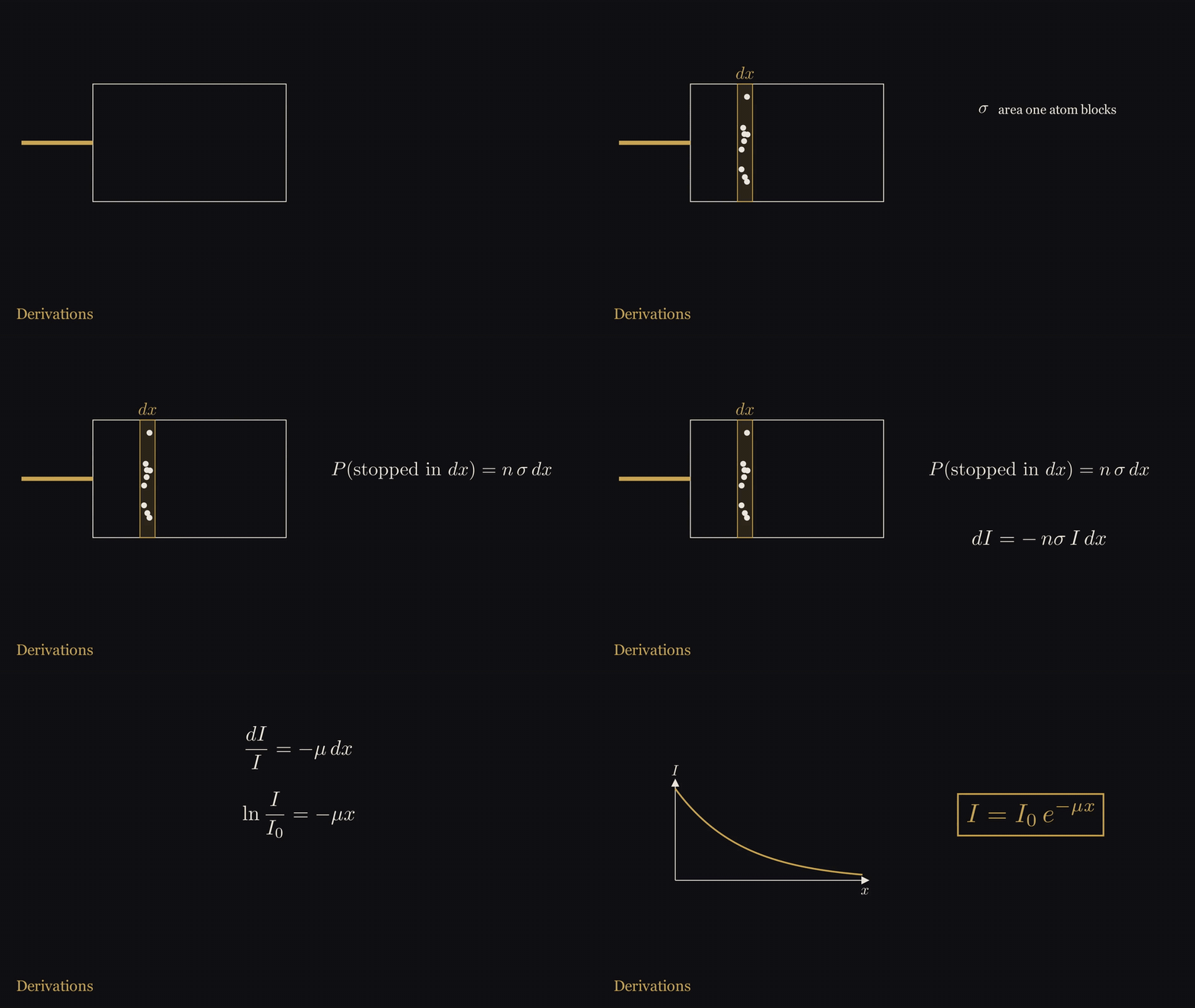
$The fraction stopped in a thin layer dx is nσ dx; integrating gives I = I₀ e^(−μx).$

Figure 8. The fraction stopped in a thin layer dx is nσ dx; integrating gives I = I₀ e^(−μx).

Definition A3.1 (cross section and number density). Suppose a material has $n$ atoms per cubic centimeter; $n$ is called the number density. The likelihood that a photon interacts with a given atom is equivalent to that atom blocking an area $\sigma$ : every photon that falls into this area is absorbed or scattered away. $\sigma$ is called this atom’s cross section for photons of that energy.

Proposition A3.2 (Beer–Lambert law). A narrow, parallel beam of monoenergetic X-rays enters a uniform material perpendicularly. Let $I(x)$ be the number of photons at depth $x$ that have not yet undergone any interaction. Then

I(x) = I_0\,e^{-\mu x}, \qquad \mu = n\sigma. \tag{A3.1}

Proof. At depth $x$ take a thin slice of thickness $dx$ and area $S$ . The slice contains $nS\,dx$ atoms, and the total area they block is $nS\,dx\cdot\sigma$ . When the slice is thin enough, these small areas do not overlap, so the probability that a photon reaching this point interacts in this layer is $n\sigma S\,dx/S = n\sigma\,dx$ . Of the $I(x)$ photons reaching this layer, on average $I(x)\,n\sigma\,dx$ are blocked, so

dI = -\mu I\,dx, \qquad \mu = n\sigma.

Separating variables, $dI/I = -\mu\,dx$ ; integrating both sides from $0$ to $x$ gives $\ln(I/I_0) = -\mu x$ , which is (A3.1). (QED)

Remark A3.3. Both conditions, “narrow beam” and “monoenergetic”, matter. With a broad beam, some of the photons scattered aside still reach the detector, and the measured intensity is higher than (A3.1). A real tube emits a whole continuous spectrum; the low-energy part is eaten up first in the material, and the average energy of the transmitted beam gets higher and higher; this is called beam hardening. The examples below are all computed for a single energy.

Definition A3.4 (half-value layer). The thickness needed to halve the intensity; from $e^{-\mu x_{1/2}} = 1/2$ one gets

x_{1/2} = \frac{\ln 2}{\mu}. \tag{A3.2}

Definition A3.5 (mass attenuation coefficient). $\mu$ is proportional to density: compress the same substance to twice the density, and there are twice as many atoms per unit volume. Dividing out the density gives a quantity $\mu/\rho$ that depends only on composition and photon energy, in cm $^2$ /g. This is what the NIST tables give.

Proposition A3.6 (mixture rule). For a material composed of several elements, with the mass fraction of the $i$ -th element being $w_i$ ,

\frac{\mu}{\rho} = \sum_i w_i\left(\frac{\mu}{\rho}\right)_i. \tag{A3.3}

Proof. Per cubic centimeter, the $i$ -th element has $\rho w_i$ grams, with number of atoms $n_i = \rho w_i N_A/A_i$ . Assuming each kind of atom blocks light on its own, without affecting the others, the derivation of (A3.1) holds for each kind of atom separately, and the total $\mu = \sum_i n_i\sigma_i = \rho\sum_i w_i\,(N_A\sigma_i/A_i)$ . For a pure element $(\mu/\rho)_i = N_A\sigma_i/A_i$ ; substituting and dividing both sides by $\rho$ gives (A3.3). (QED)

“Without affecting the others” ignores the effect of chemical bonds on the outer electrons; near absorption edges there are small deviations, and away from absorption edges this approximation is very good.

Example A3.7. First look at a photon energy of 20 keV. Soft tissue: $\mu/\rho = 0.8230$ cm $^2$ /g, density 1.06 g/cm $^3$ , $\mu = 0.872$ cm $^{-1}$ , 1 centimeter thick transmits $e^{-0.872} = 41.8\%$ ; cortical bone: $\mu/\rho = 4.0010$ cm $^2$ /g, density 1.92 g/cm $^3$ , $\mu = 7.68$ cm $^{-1}$ , 1 centimeter thick transmits only $e^{-7.68} = 0.046\%$ . The 42% and 0.05% in the main text are these two numbers. Next look at a photon energy of 30 keV. Soft tissue: $\mu/\rho = 0.379$ cm $^2$ /g, density 1.06 g/cm $^3$ , $\mu = 0.402$ cm $^{-1}$ , half-value layer $x_{1/2} = 0.693/0.402 = 1.73$ cm. After passing through 10 centimeters of soft tissue, $e^{-4.02} = 1.8\%$ is left. Cortical bone: $\mu/\rho = 1.331$ cm $^2$ /g, density 1.92 g/cm $^3$ , $\mu = 2.56$ cm $^{-1}$ , half-value layer only 0.27 cm.

Example A3.8 (reproducing the NIST table with the mixture rule). The composition of cortical bone given by NIST (mass fractions) is: hydrogen 3.4%, carbon 15.5%, nitrogen 4.2%, oxygen 43.5%, sodium 0.1%, magnesium 0.2%, phosphorus 10.3%, sulfur 0.3%, calcium 22.5%. Summing the nine elements’ individual $\mu/\rho$ with weights according to (A3.3) gives 1.3309 cm $^2$ /g at 30 keV; the value for cortical bone in the NIST table is 1.3310. Taking nine energy points from 20 keV to 1 MeV, for both materials, bone and soft tissue, the weighted results differ from the values in the table by no more than 0.04% in every case. This shows only that we reproduced the way NIST compiled its tables, because NIST computed the values for compounds with this very rule in the first place; to test the rule itself, one would have to compare with measured attenuation coefficients of bone, which this appendix has not done.

A.4 Bone and flesh

The electrons in an atom are held by the nucleus; the minimum energy needed to take an electron out of the atom is called its binding energy; the farther inside the shell an electron is, the larger its binding energy. When photons pass through matter, in the energy range from a few tens of keV to 1 MeV there are mainly three interactions:

Photoelectric effect: the photon is absorbed by the atom as a whole and knocks out an inner-shell electron. The photon energy must be higher than the binding energy of this electron.
Incoherent scattering, also called Compton scattering: the photon hits an electron, hands part of its energy to it, and changes its own direction. When the photon energy is far above the binding energy, the electrons in the atom can be treated as free electrons.
Coherent scattering, also called Rayleigh scattering: the photon is bounced off by the atom as a whole, with its energy unchanged, changing only its direction.

When the energy exceeds 1.022 MeV (twice the electron rest energy), electron–positron pairs are also produced, which this appendix does not need. Adding the three parts:

\frac{\mu}{\rho} = \left(\frac{\mu}{\rho}\right)_{\text{photoelectric}} + \left(\frac{\mu}{\rho}\right)_{\text{coherent}} + \left(\frac{\mu}{\rho}\right)_{\text{incoherent}}. \tag{A4.1}

Proposition A4.1 (high-energy limit: only density and electron count remain). If at some energy incoherent scattering is overwhelmingly dominant, and the cross section $\sigma_e$ per electron does not depend on which kind of atom it belongs to, then

\frac{\mu}{\rho} \approx N_A\,\sigma_e\,\langle Z/A\rangle, \qquad \frac{\mu_{\text{bone}}}{\mu_{\text{flesh}}} \approx \frac{\rho_{\text{bone}}}{\rho_{\text{flesh}}}\cdot\frac{\langle Z/A\rangle_{\text{bone}}}{\langle Z/A\rangle_{\text{flesh}}}. \tag{A4.2}

where $N_A\langle Z/A\rangle$ is just the number of electrons per gram of material.

Proof. The $i$ -th kind of atom has $Z_i$ electrons, each with cross section $\sigma_e$ , so $\sigma_i = Z_i\sigma_e$ , $(\mu/\rho)_i = N_A\sigma_i/A_i = N_A\sigma_eZ_i/A_i$ . Substituting into the mixture rule (A3.3) gives the first formula. Comparing two materials, $N_A\sigma_e$ cancels, and multiplying by the density factor of $\mu = \rho\cdot(\mu/\rho)$ gives the second formula. (QED)

Example A4.2. Computed from the NIST compositions, cortical bone has $\langle Z/A\rangle = 0.51478$ , soft tissue $0.54996$ , a ratio of 0.9360. Hydrogen’s $Z/A$ is close to 1 and all the other elements are close to 0.5; soft tissue contains 10.2% hydrogen, bone only 3.4%, so a gram of soft tissue actually has more electrons than bone. The density ratio is $1.92/1.06 = 1.8113$ . By (A4.2), in the high-energy limit the ratio of the linear attenuation coefficients of bone and flesh is $1.8113\times0.9360 = 1.6954$ . The ratio given by the NIST table at 1 MeV is 1.6976, 0.12% higher than predicted. Broken down: the ratio of the incoherent parts of the two materials is 0.04% lower than the ratio of electron counts, and at 1 MeV the bit of coherent scattering and photoelectric effect that remains raises the total ratio by 0.16%.

Example A4.3 (how much each of the three parts contributes). Looking up each element’s cross sections for the three parts individually in NIST’s XCOM database, then weighting according to (A3.3), gives the table below. “Photoelectric share” is the proportion of the photoelectric part in the total $\mu/\rho$ .

Energy	Bone: photoelectric share	Flesh: photoelectric share	Linear attenuation coefficient ratio, bone/flesh
20 keV	92%	68%	8.80
30 keV	81%	40%	6.36
50 keV	52%	13%	3.39
100 keV	14%	2%	1.99
150 keV	5%	1%	1.80
1 MeV	0%	0%	1.70

The ratio falls all the way from 8.8 to 1.70, and the fall goes in step with the fading of the photoelectric share.

Example A4.4 (what the extra part at low energy is). At 20 keV the ratio 8.80 is about 5.2 times the high-energy limit 1.70. Scaling each part of soft tissue by “the ratio of incoherent scattering” onto the same electron-count basis as bone, bone has an extra 3.28 cm $^2$ /g. Broken down, 97% of this comes from the photoelectric effect and 3% from coherent scattering. At 30 keV it is 95% and 5%. The main text says the extra part comes from the photoelectric effect; according to the data this is broadly so, though strictly a few percent also comes from coherent scattering.

Empirical scaling A4.5 (how strongly the photoelectric effect favors heavy atoms). Deriving the photoelectric cross section theoretically requires quantum mechanics; we do not do it here, but only read the exponents off NIST’s table of photoelectric cross sections. This table itself was computed by Scofield in 1973 with the Dirac equation. Converting the per-gram $\mu/\rho$ into a per-atom cross section $\sigma = (\mu/\rho)\,A/N_A$ :

At 30 keV, calcium has $\sigma_{\text{photoelectric}} = 248$ b and oxygen $4.36$ b, a factor of 57 apart; the ratio of the atomic numbers of calcium and oxygen is $20/8 = 2.5$ , and $2.5^{4.41} = 57$ . Phosphorus against carbon gives an exponent of 4.54. At 60 keV the two exponents are 4.57 and 4.68.
As the energy rises from 20 keV to 60 keV (three times), the photoelectric cross section of oxygen falls to $3^{-3.27}$ of its value, and that of calcium to $3^{-3.04}$ .

Putting these together, in this energy range, per atom roughly

\sigma_{\text{photoelectric}} \propto \frac{Z^{4.4\sim4.7}}{E^{3.0\sim3.3}}. \tag{A4.3}

The number of atoms per gram of material is roughly proportional to $1/A \approx 1/(2Z)$ , so per gram the exponent of $Z$ has 1 subtracted, giving roughly between 3.4 and 3.7. In bone, calcium accounts for 22.5% and phosphorus for 10.3%, and the photoelectric effect is so sensitive to $Z$ , so at low energies bone blocks especially much.

Remark A4.6 (absorption edge). NIST’s cortical bone table lists two values at the single energy 4.0381 keV, 129.6 and 333.2 cm $^2$ /g, a jump by a factor of 2.57. This energy is exactly the binding energy of the innermost (K-shell) electrons of the calcium atom. When the photon energy is below it, calcium’s two K-shell electrons cannot take part in the photoelectric effect; as soon as it is above it, these two electrons join in, and absorption suddenly becomes stronger. This is called the K absorption edge. The characteristic lines in Section A.5 below are the light emitted when, after a vacancy has been knocked out of the K shell, an outer electron jumps down to fill it.

Remark A4.7 (the glass tube wall absorbs its own characteristic lines). The light emitted when a vacancy appears in an atom’s K shell and an outer electron fills it has an energy determined by the element, and is called that element’s characteristic line (see A.5 for details). The main text says that the characteristic lines of the light elements in the glass are absorbed by the tube wall; this can be computed with (A3.1). The composition of the glass of Röntgen’s tube is not known; here borosilicate glass (density 2.23 g/cm $^3$ ), for which NIST has data, is used as the absorber. In the NIST X-ray transition energies database, the measured energies of the strongest K-series line of several common glass elements are: sodium 1.041 keV, silicon 1.740 keV, potassium 3.314 keV, calcium 3.692 keV. Of these, the calcium line has the highest energy and penetrates most easily; as long as the tube wall is thicker than 0.11 millimeters, less than a thousandth of it remains; at 0.5 millimeters, $6\times10^{-15}$ remains, and the other lines even less. Through the same 0.5 millimeters, the continuous spectrum at 20 keV is 77% transmitted, at 30 keV 92%. Borosilicate glass is only a substitute. Redoing the calculation with soda-lime glass, the most common today, shows which way the error caused by the substitute goes. Using a typical composition of soda-lime container glass (silica 74%, sodium oxide 13%, calcium oxide 10.5%, the rest small amounts of alumina, potassium oxide and magnesium oxide; density 2.52 g/cm $^3$ ), soda-lime glass is heavier than borosilicate glass and also contains calcium, and it absorbs more at all four lines and both energies computed above. In soda-lime glass, only 0.093 millimeters are needed for less than a thousandth of the four characteristic lines to remain, so the conclusion only holds more strongly; the transmission of the continuous spectrum would be lower, at 0.5 millimeters 67% at 20 keV and 87% at 30 keV. This conclusion applies only to glass that contains no heavy elements. If the tube was made of lead glass, or fitted with a metal target such as platinum, the characteristic lines of the heavy elements have much higher energies and may get through; that would have to be computed separately.

A.5 Preview: two things later episodes will cover

Characteristic lines and Moseley’s law. In the model of the hydrogen atom that Bohr gave in 1913, the electron can only be in discrete orbits, one shell after another, and the energy of the $n$ -th shell is $-R_y/n^2$ , $R_y = 13.606$ eV. An ion with only one electron and nuclear charge $Z$ is called a hydrogen-like atom, with energy $-R_yZ^2/n^2$ . Now knock out one electron from the innermost shell ( $n=1$ ) of an atom, leaving a vacancy; an electron from the next shell out ( $n=2$ ) jumps down to fill it and emits a photon, and this line is called K $_\alpha$ . Roughly speaking, the nuclear charge felt by the electron jumping down is screened by about one unit by the one electron remaining in the K shell, equivalent to a hydrogen-like atom with atomic number $Z-1$ . This is only an empirically useful estimate: strictly speaking, the electrons of the two shells are not screened the same way, and taking the same $Z-1$ works partly through a lucky cancellation. Thus

E_{K_\alpha} \approx R_y(Z-1)^2\left(1-\frac14\right) = \frac34R_y(Z-1)^2. \tag{A5.1}

$\sqrt{E}$ is linear in $Z$ . This straight line later became the basis for lining up the elements by atomic number.

Example A5.1. Comparison with NIST’s measured values (the strongest line within K $_\alpha$ ):

Element	$Z$	Computed from (A5.1)	Dirac equation, nuclear charge taken as $Z-1$	NIST measured
Copper	29	8.000 keV (−0.6%)	8.107 keV (+0.7%)	8.048 keV
Molybdenum	42	17.15 keV (−1.9%)	17.66 keV (+1.0%)	17.48 keV
Tungsten	74	54.38 keV (−8.3%)	60.08 keV (+1.3%)	59.32 keV

Copper agrees very well; tungsten is off by 8%. According to the Bohr model, the speed of an innermost electron is about $Z\alpha c$ : for copper $0.21c$ , for tungsten $0.54c$ , where the nonrelativistic formula can no longer be used. The Dirac equation is the relativistic quantum equation for the electron; computing the same hydrogen-like model with it instead pulls the inner energy levels deeper, and the tungsten discrepancy shrinks from −8.3% to +1.3%. So the discrepancy of (A5.1) for heavy elements is mainly caused by relativistic effects.

Bragg condition. The atoms in a crystal are arranged in neat order and can be seen as layer upon layer of parallel planes; the spacing between adjacent layers is written $d$ . A beam of X-rays of wavelength $\lambda$ comes in at a glancing angle $\theta$ (the angle between the ray and the crystal plane), and each layer of atoms scatters part of it out.

Proposition A5.2 (Bragg condition). Looking only at the direction where the outgoing angle equals the incoming angle (as in mirror reflection), the condition for the outgoing waves from adjacent layers to reinforce each other in phase is

2d\sin\theta = n\lambda, \qquad n = 1, 2, 3, \dots \tag{A5.2}

Proof. First look at the atoms within one layer. When the outgoing angle equals the incoming angle, the waves scattered from any two atoms on the same layer travel the same total path, so all the scattering from one layer is in phase, and the layer acts like a mirror. Next look at two adjacent layers. Take a point $P$ on the upper layer and the point $Q$ directly below it on the lower layer, $PQ = d$ , perpendicular to the crystal planes. The ray reflected via $Q$ travels two extra segments compared with the ray reflected via $P$ : drop a perpendicular from $P$ to the incoming ray through $Q$ , and the distance from its foot to $Q$ is $d\sin\theta$ ; likewise on the outgoing side, it is also $d\sin\theta$ . So the path difference is $2d\sin\theta$ . When it equals an integer multiple of the wavelength, the reflected waves of the two layers meet crest to crest and reinforce each other; this holds for every pair of adjacent layers, so the reflections of all the layers reinforce together. When the path difference is not an integer multiple, the phases of the reflections of successive layers are shifted step by step, and with very many layers, they cancel each other when added up. (QED)

Example A5.3. A crystal is built up from identical small cubic cells, and the edge length of a small cell is called the lattice constant. The lattice constant of sodium chloride is $a = 564.02$ pm. Take the set of crystal planes parallel to the cube faces, with spacing $d = a/2 = 282.0$ pm, and use copper’s K $_\alpha$ line, $\lambda = hc/E = 1239.842/8047.82 = 0.15406$ nm. By (A5.2), $\sin\theta = n\lambda/2d$ : for $n = 1$ , $\theta = 15.85°$ ; for $n = 2$ , $33.11°$ ; for $n = 3$ , $55.03°$ . $n\lambda/2d$ cannot exceed 1, so this set of planes has at most three orders of reflection.

Remark A5.4. Why are crystals used for diffraction of X-rays, but not of visible light? (A5.2) requires $\lambda \le 2d$ . The spacing of crystal planes is a few tenths of a nanometer, and the wavelength of X-rays is also a few tenths of a nanometer, a perfect match; the wavelength of visible light is seven hundred to twelve hundred times $2d$ , and no angle can satisfy the condition. Why take $a/2$ rather than $a$ : in sodium chloride, exactly halfway between two planes spaced $a$ apart there is another plane of exactly the same composition, half sodium and half chlorine. For the first-order reflection calculated with spacing $a$ , the wave reflected back by this intervening plane lags by exactly half a wavelength and cancels it. So within this family of planes parallel to the cube faces, the first reflection that can be seen comes from the planes with spacing $a/2$ . In other directions there are other planes, for example the set along the cube diagonal with spacing $a/\sqrt3 = 325.6$ pm, where sodium layers and chlorine layers alternate; its first-order reflection is at $13.68°$ , even earlier than the $15.85°$ above, but the reflections from sodium and chlorine largely cancel each other, so it is very weak.

Data sources for this appendix. NIST X-ray Mass Attenuation Coefficients (J. H. Hubbell and S. M. Seltzer; Tables 1, 2 and 4, the three material tables for cortical bone, soft tissue and borosilicate glass, and Chapter 2, which describes how the tables were compiled); the NIST XCOM photon cross sections database, queried element by element; the NIST X-ray Transition Energies database, taking the strongest line within K $_\alpha$ (recorded in the database as KL $_3$ ), direct experimental values; Feynman, The Feynman Lectures on Physics, Volume I, Chapter 32; the lattice constant of sodium chloride is taken from the Wikipedia article “Sodium chloride”, and the composition and density of soda-lime glass from the Wikipedia article “Soda–lime glass” (container glass column). Every number computed from these data was computed by the script verify_appA.py, and the original web pages were archived as well. The wavelength range of visible light, the size of atoms, and the 1.022 MeV threshold for pair production are general knowledge and were not separately checked; the tube wall thickness of 0.5 millimeters is an assumption used for illustration.

References

Numbered in order of first appearance in the main text. [primary] = original documents, newspapers and periodicals of the time, or institutions’ own catalogue records; [secondary] = later research or retellings.

W. C. Röntgen, Ueber eine neue Art von Strahlen (Vorläufige Mittheilung), Sitzungs-Berichte der Physikalisch-Medicinischen Gesellschaft zu Würzburg, 1895, pp. 132–141 (MDZ bsb11565199); separate offprint (Stahel, Wellcome b30475697, public domain) [primary]: https://www.digitale-sammlungen.de/en/view/bsb11565199?page=136
German Röntgen Museum, museum-digital 7536 (paper print from the Zehnder collection); Wellcome Collection 32971i (item from the Schuster collection); Science Museum Group A606881 [primary, institutional catalogue record]: https://rheinland.museum-digital.de/object/7536
O. Glasser, Wilhelm Conrad Röntgen and the Early History of the Roentgen Rays (1945), p. 40 [secondary]
Nature 53 (1896-01-23), pp. 274–276 (Stanton’s English translation and figure) [primary]: https://archive.org/details/sim_nature-uk_1896-01-23_53_1369/page/n11/
Minutes of the meeting of the Würzburg Physical-Medical Society on January 23, 1896, Sitzungs-Berichte 1896, p. 11 (archive.org bub_gb_cPgyAQAAMAAJ) [primary]: https://archive.org/details/bub_gb_cPgyAQAAMAAJ/page/n18/
NIST X-ray Mass Attenuation Coefficients (ICRU-44 cortical bone, soft tissue), computed by Abel (verify_1901.py, verify_appA.py) [primary data]: https://www.nist.gov/pml/x-ray-mass-attenuation-coefficients
Official Nobel Prize: facts page and citation for the 1901 Physics Prize; Röntgen biography (from Les Prix Nobel); presentation speech (C. T. Odhner); Röntgen lecture page (“No Lecture was delivered by Professor W. Röntgen.”). nobelprize.org [primary]: https://www.nobelprize.org/prizes/physics/1901/rontgen/facts/ · https://www.nobelprize.org/prizes/physics/1901/ceremony-speech/ · https://www.nobelprize.org/prizes/physics/1901/rontgen/lecture/
Folke Henschen, “From the first Nobel Prize award ceremony 1901” (1976 recollection), nobelprize.org [primary, eyewitness]: https://www.nobelprize.org/ceremonies/from-the-first-nobel-prize-award-ceremony-1901/
Röntgen’s letter of 1901-12-06 to the Bavarian Ministry of Culture and Education requesting leave, English translation in the University of Würzburg’s 2020 exhibition catalogue, p. 52 [primary, quoted via a secondary]
Nomination archive, Physics Prize 1901 (30 records, 1 of which is misfiled) [primary]: https://www.nobelprize.org/nomination/archive/list.php?prize=1&year=1901
P. Lenard, On Cathode Rays, Nobel lecture, 1906-05-28, nobelprize.org [primary]: https://www.nobelprize.org/prizes/physics/1905/lenard/lecture/
O. Glasser, Cleveland Clinic Quarterly 20(3): 400–406 (1953), quoting Lenard’s 1929 letter and 1945 conversation [primary, quoted via a secondary]: https://www.ccjm.org/content/ccjom/20/3/400.full.pdf
M. Treutwein, Röntgen’s last will, Physics and Imaging in Radiation Oncology 28:100503 (2023) [primary]: https://doi.org/10.1016/j.phro.2023.100503
Nobel Foundation, Prize amount and market value of invested capital (2023 edition) [primary]: https://www.nobelprize.org/uploads/2023/04/prize-amounts-2023-2.pdf
Letter from Marion & Co. of 1896-01-06, held by the German Röntgen Museum (museum-digital catalogue record) [primary, institutional catalogue record]
Die Presse (Vienna), 1896-01-05, front page, “Eine sensationelle Entdeckung” (ÖNB ANNO apr18960105) [primary]: https://anno.onb.ac.at/cgi-content/anno?aid=apr&datum=18960105&seite=1
Wiener klinische Wochenschrift 9 (1896), Nr. 5, pp. 82–83: minutes of the meeting of the Society of Physicians in Vienna on 1896-01-24, von Mosetig-Moorhof’s report (archive.org wienerklinischew09unse) [primary]: https://archive.org/details/wienerklinischew09unse/page/n99/
Montreal Medical Journal 24 (1896), pp. 664–665 (Cox; Kirkpatrick) and accompanying figure; editorial in the same volume, May 1896, The New Photography (archive.org montrealmedicalj24mont) [primary]: https://archive.org/details/montrealmedicalj24mont/page/n687/
Life (New York) 27, no. 687 (1896), p. 155, cartoon The New Roentgen Photography. “Look pleasant, please.” [primary]: https://archive.org/details/sim_life_1896-02-27_27_687/page/n6/
Plainfield Daily Press (New Jersey), 1896-02-18; American Journal of Photography, March 1896, p. 98 [primary]: https://archive.org/details/ppl-dailyp_1896-02/page/n115/ · https://archive.org/details/sim_american-journal-of-photography_1896-03_17_195/page/n5/
O. Glasser, Wilhelm Conrad Röntgen und die Geschichte der Röntgenstrahlen (Springer, 1931), appendix pp. 296–337: bibliography of publications of 1896 (books nos. 1–49, articles nos. 50–1044) [primary, bibliography]
Electrical Review (New York) 28, no. 22 (1896-05-27), p. 274; Scientific American 74, no. 22 (1896-05-30), p. 339 [primary]: https://archive.org/details/sim_factory_1896-05-27_28_22/page/n5/ · https://archive.org/details/sim_scientific-american_1896-05-30_74_22/page/n2/
J. Daniel, The X-rays, Science N.S. 3, no. 67 (1896-04-10), pp. 562–563 [primary]: https://archive.org/details/sim_science_1896-04-10_3_67/page/n25/
New York Times, 1903-08-03, p. 3; 1904-10-04, p. 16; The Fulton County News (McConnellsburg, Pennsylvania), 1903-08-05, p. 2, Had enough of the X ray (reprinted from New York, including the words of Dally’s doctor, Graves) [primary]: https://archive.org/details/sim_new-york-times_1903-08-03_52_16716/page/n2/ · https://archive.org/details/sim_new-york-times_1904-10-04_54_17083/page/n15/ · https://archive.org/details/per_the-fulton-county-news_the-fulton-county-news_1903-08-05_1/page/n1/