[Author’s note — Yeqiu]
When we ask whether an AI’s proof is reliable, behind that question there is in fact a bigger one: why is a proof that we have not verified ourselves reliable? Our usual answer is probably something like peer review, verifiability and so on. But when we measure AI’s proofs by the same standard, we run into a question that cannot be avoided: is AI a peer? Or rather, is AI qualified to be a peer?
And the word “qualified” may be heavier than it looks. A peer is not just someone capable enough; a peer is someone who makes mistakes and has to answer for their own mistakes: staking a reputation, staking a career. AI, by contrast, has nothing it can lose. This chain of questions is probably hard to answer to this day even for the top scientists in the field. But it is not far away; it is a question our present era is facing, and it is closely bound up with how we actually use AI.
I don’t have an answer. But it is exactly this question without an answer that pushes me toward another, inward-looking question: in such an era, how should a person conduct themselves?
In the author’s notes of earlier installments I mentioned that in the AI era, reading books will become more important, not less. Because in this era, reading is a personal experience, and it is also the foundation on which a person forms their own thought. And personal experience will become more and more important, because AI is changing this era very fast; if we still measure people and AI by the old standards, such as how much code one has written, how much knowledge one has stored, how efficiently one completes tasks, then people are bound to be at a disadvantage.
But what is truly unique and irreplaceable about people comes precisely from our personal experience, from the experience, thought and feeling formed by that experience; if they benefit another person or let another person feel the same, that moment is happiness.
Episode 7 of the series. In the previous episode we opened the box holding the 26 sporadic simple groups, watched them come on stage one after another across several decades, and said: all these sporadic groups in the end point faintly toward the same monster, unreasonably large. In this episode we look at this monster head-on (it has a formal name, the Monster): how it was first “computed” and then “built” by one person by hand. It lives in 196883 dimensions. And why does 196884 (exactly 1 more than 196883) appear almost unchanged in a seemingly unrelated corner of number theory? That crack is left for the last episode.
“317 is a prime, not because we think so, or because our minds are shaped in one way rather than another, but because it is so, because mathematical reality is built that way.”
— G. H. Hardy (1877–1947), A Mathematician’s Apology §24
Companion video (YouTube)
Prelude · First the medical report, then the thing itself
There is a rare thing in the history of mathematics, and it happened precisely to the protagonist of this episode: before anyone saw this monster, mathematicians had already written its medical report: how big it is, what its “fingerprint table” looks like, the minimum number of dimensions of the space it has to live in, all of it had been computed. Then several more years passed before someone actually built it, confirmed its identity, and matched it point by point against the report written in advance.
An object’s medical report existing before the object itself: in other fields this is almost unimaginable. It is hard to measure an animal’s height and weight first and then go back and discover the animal. But this is exactly how the Monster came on stage: first the numbers, then the thing. What this episode tells is how this report was computed (§1, §2), how the person who really put the monster up completed it by hand (§3), and finally we take stock: is there anything else left in the box at all (§4)?
§1 · Fischer’s mirrors
One end of the story is in Germany in the 1960s. Bernd Fischer (1936–2020), a group theorist who later led mathematics at the University of Bielefeld, asked a question that looked too plain to lead to a monster.
 Bernd Fischer (1936–2020): his plain question, “mirrors may only meet at or ”, led in the end to the Monster. (Photo by Katrin Breithaupt, 2008, Oberwolfach Photo Collection, CC BY-SA 2.0 de.)
To explain this question clearly, we first have to talk about the person who led him onto this road. In secondary school Fischer had an excellent mathematics teacher, who before World War II had spent three years as an assistant in Darmstadt computing rocket trajectories (that was exactly the era in which Germany led in rockets; the V2 came out of the late phase of World War II), with real, hands-on differential equations. But this teacher was not a rocket expert; he was a mathematician; and what really moved Fischer was not the rockets, but his way of using mathematics to handle physical problems. How good was he? After Fischer went to university, he did not need to attend a single lecture of the differential equations course. Influenced by this teacher, his plan on entering university was to do a master’s in physics first and then a doctorate in mathematics; in other words, he had originally meant to go into applied mathematics.
 Reinhold Baer (1902–1979): the teacher who led Fischer from “would-be applied mathematician” to pure mathematician; when teaching analysis he would deliberately make mistakes and wait for the students to correct him. (Photo by Konrad Jacobs, Oberwolfach Photo Collection, CC BY-SA 2.0 de.)
But the one who led him toward another road was Reinhold Baer, a professor who had just returned to Germany from the United States. What fascinated Fischer was not the content of some particular course, but Baer’s way of doing mathematics, and his way of talking to these young students. The example Fischer gives is: when Baer taught analysis he would deliberately make mistakes and wait for the students to correct him, an act that made “you are entitled to question me” an everyday thing. He admired Baer for two more things: first, breadth, wanting to bring every direction into the seminar; second, freedom: you could do whatever you wanted, which was very unusual in German universities at the time. These things together turned a would-be applied mathematician into a pure mathematician. Baer’s seminar also drew almost everyone in this field to Frankfurt: Tits (Jacques Tits, 1930–2021) came often, Thompson (John Thompson, 1932–) came, and Janko (Zvonimir Janko, 1932–2022) came too.
And Fischer himself recalled that one of the things he read after burrowing into the library as a student was a structure called a “distributive quasigroup”; he felt at the time that there was plainly a group hidden behind it. This later became exactly the topic of his doctoral thesis, and exactly the starting point that led him onto the road of “groups generated by mirror-like operations”.
Fischer’s question. Imagine a batch of operations, each one like a mirror: reflect once, left and right are flipped; reflect twice, back to how it was (such an element that “returns to the original after multiplying by itself once” is called an involution in mathematics; we already dealt with it in EP5). What Fischer wanted to study were groups generated by a whole class of such “mirrors”; but he added a very tight restriction: take any two mirrors and reflect in them one after the other; the order of this composite operation may only be 1, 2 or 3, nothing larger.
Translated into geometry, this restriction is a very clean sentence. Reflecting in two mirrors one after the other composes to a rotation, whose angle is exactly twice the angle between the two mirrors. So “the order of the composite operation is at most 3” is the same as saying: any two mirrors either coincide, or meet at 90°, or meet at 60°, and no other angle is allowed. The whole group then becomes a huge network of mirrors, and what Fischer asked was: how many kinds of such networks can there be in all?
The answer is abnormally short. Fischer proved around 1970: the “atoms of symmetry” (which can be understood as the simple groups that cannot be divided further) satisfying these rules come in exactly six classes. Five of them are long-familiar faces: all rearrangements ; three families of classical groups over (the smallest field, with only the two elements and ): the symplectic groups , the unitary groups , the orthogonal groups (these three families all grow on the Killing–Cartan periodic table of EP4, and the Chevalley recipe told in EP5 §1 is the procedure that carries them over from the real numbers to finite fields: the symplectic groups are the family on the table, which is what EP4 called them; the orthogonal groups are the / families, which EP4 wrote as on the real-number side; the unitary groups are a branch twisted out of the family, which EP5 Appendix D even constructed explicitly); plus one family of orthogonal-type groups over . And the sixth class is three brand-new sporadic groups that nobody had seen before, today written , , . (For the structure of this classification, and an example you can compute by hand ( itself is a network of mirrors), see Appendix A.)
A warning bell has to be struck here, one already planted at the end of EP6: Fischer’s and Mathieu’s from the previous episode are two different families. Fischer, to save trouble back then, wrote these three groups as , , , deliberately echoing Mathieu; only when the big atlas was published in 1985 were they uniformly changed to (the first two letters of Fischer), to avoid a name clash with the Mathieu groups. The same subscripts, completely different groups, and sizes that differ by an enormous distance: the order of Mathieu’s is 443,520, while Fischer’s is about , about one hundred fifty million times larger.
Loosen the mirror rule by one notch, and you are on the road to the Monster. After Fischer stepped down as dean and returned to research, he loosened the restriction from “angles may only be 90°/60°” to also allowing 45° (corresponding to composite operations of order up to 4). Why 4, and not larger? There is no limit given by mathematics here: that was the step Fischer took at the time, and it succeeded. Pushing the same idea of mirror networks further, in the summer of 1973 he caught the largest group among them, which Conway (John Conway, 1937–2020) later named the Baby Monster. How big is it? Its order is
About this number there is a true little episode: Fischer was visiting Cambridge, and Conway wanted to use an old mechanical calculator to help him compute the last step, but could not find the missing part however he looked, and in the end Fischer and his wife simply finished it by hand. Fischer said he had something to go on: he knew the answer had to be divisible by 31, so the computation came with a built-in check. In August of that year, at the meeting in Oberwolfach, he spoke publicly about this new group for the first time.
The lecture register of this meeting still survives: the Oberwolfach institute’s Vortragsbuch, volume 25, page 58, with the meeting dates handwritten as 5. 8. 73 – 10. 8. 73, the title {3,4}-Transpositions in finite groups, and below it Fischer’s own signature. And the abstract he wrote is itself a question:
Is there a finite simple group satisfying …
What follows is the prime factorization of the 33-digit number above. This page makes the word “prediction” solid: at that moment, this group really was still only a question with a precise order.
And right around the time he computed the Baby Monster, Fischer and another person realized almost at the same time: this colossus was very likely only a cross-section of some larger group. That “larger group” is the Monster: at this moment it was predicted for the first time.
§2 · The atlas and the report written in advance
The moment of prediction. At the end of 1973, Fischer noticed that his huge group might be embedded in a larger group; almost at the same time, Robert Griess (1945–) in Michigan, in the United States, independently arrived at the same idea. Both were convinced: there should exist a larger simple group, with the Baby Monster inside it. As for how big it actually was, nobody knew. This is the moment the Monster was “predicted”: people first became convinced that it should exist and how big it should be, while nobody had yet seen it.
In the next few years, what mathematicians did was give this monster, which had not yet shown itself, a medical examination. And the reason this could be done rested on a big book that was being compiled, and a few iron laws about “the fingerprint of a group”.
That big book is called the ATLAS of Finite Groups. The idea arose around 1970 in Cambridge: Conway discovered a huge new group in 1969 (coming from a structure called the Leech lattice, told in EP6), and then spent more than a year working out its properties and computing its fingerprint table; this gave him an idea: simply compile a handbook listing all the interesting properties of all the interesting groups. The book was finally compiled by five people: Conway, Curtis (Robert Curtis), Norton (Simon Norton), Parker (Richard Parker), Wilson (Robert Wilson); it was published by Oxford University Press in 1985, having taken about fifteen years altogether. (An Easter egg only group theorists will smile at: these five surnames all happen to have six letters.)
 John Thompson (1932–): his “order formula” can work back from the neighbor circle of an involution to the order of the whole group, and it was the key tool for weighing the Monster. (Photo by Renate Schmid, 2007, Oberwolfach Photo Collection, CC BY-SA 2.0 de.)
The order of the Monster was computed. Weighing such a group that has not yet been built uses a clever tool, the Thompson order formula (invented by Thompson, the group theorist of EP5 and EP6): it can work back from the “centralizer” of an involution (all the elements that commute with it) to the order of the whole group.
This step is worth pausing on. Look closely at what it takes in and what it puts out: what it takes in is only the “neighbor circle” of an involution, the subgroup formed by those elements that commute with it under multiplication; what it puts out is the order of the whole group, an exact integer. It needs only one premise: the involutions of this group fall into exactly two classes; and the Monster has exactly two classes. So what has to be taken in is the neighbor circle of each of these two classes, and no other input is needed beyond that.
The numbers on the Monster’s side make the gap clear. Its involutions fall into two classes; the neighbor circle of the second class (written 2B) is exactly : the Conway group from the previous episode is back. Take , already computed in EP6 ( is the half of it left after quotienting out ), and multiply by the of the outer shell; the size of this neighbor circle is
a 27-digit number. And the Monster itself is a 54-digit number: exactly twice as many digits. That is to say, the size of this neighbor circle is of the same order of magnitude as the square root of the whole Monster (in fact about one sixth of the square root); compared with each other, it is smaller by a factor of about . It is just these two small local pieces that fixed that 54-digit number without a single digit wrong.
The intuition for why this road works is that involutions are used in pairs. Take any two involutions; what they generate is always a dihedral group, the symmetry group of some regular polygon, whose number of sides is the order of their product (the lemma in Appendix A proves this, and it holds for any group). So “how big is the whole group” can be rewritten as “how many pairs of such involutions can be formed, and which dihedral block each pair falls into”. Thompson’s formula counts this out to the end; once it is counted, the sizes of the two neighbor circles are multiplied and added, and what is left is exactly . (For the shape of the formula see the end of Appendix B; for the complete proof see Appendix D: it is the cheapest proof in the whole article.)
Put it back on the main line of local analysis from EP5 §3: Brauer–Fowler 1955 (fully proved in EP5 Appendix I) says “fix the neighbor circle of an involution, and only finitely many finite simple groups fit it”, collapsing the infinite into the finite; Thompson collapsed this sentence one notch further: not finitely many, but one exact number. The same knife, sharpened a little more.
 John Conway (1937–2020): he named Fischer’s new group the “Baby Monster”, and computed the order of the Monster through the night, writing to tell Fischer at daybreak. (Photo by Thane Plambeck at the 2005 Banff conference, CC BY 2.0.)
Back to 1973. Fischer first pinned down an upper bound with two cross-sections; Conway then ran an old programmable calculator all night, got a concrete number at daybreak, tried it, and it fit. He immediately wrote to Fischer (in translation): “Dear Bernd, the order of the Monster is … but I think you already know.” In January 1974, in Oberwolfach, the order of the Monster was written down for the first time, and at that time it did not yet have a name:
(This number has 54 digits. Note that is squared and is cubed, not ordinary first powers: this point will come back later.)
Next comes that fingerprint table. Every finite group has a character table: sort the elements of the group by “same type” into a number of classes, then list all the “representations that cannot be broken down” of the group one by one, fill each cell with a number, and you get a square matrix: it is the group’s most condensed identity card. The Monster’s table has 194 rows and 194 columns, and it was computed by Fischer and Donald Livingstone, with the program written by Michael Thorne, in the 1970s: Fischer computed for a long time in Birmingham from about 1974, and it was finalized in 1979 (the years differ slightly across three sources). Remember this time: whichever year you take, the Monster had at that point still not been proved to exist. (What a character is, how this table is read, and on what grounds “computing a group’s table without having seen the group” is possible, see Appendix B: there a small table computes each of these for you.)
Credit for one thing has to be sorted out here, because it is easily mixed up: the order was fixed by Thompson’s formula, together with the combined efforts of Conway, Harada, Thompson and others; the character table was computed by Fischer, Livingstone and Thorne; as for the proof of this monster’s uniqueness, and the final proof of its existence, those were the business of other groups of people again (uniqueness was reduced by Thompson in 1979 and later completed by Griess and others; existence, that is, building it, is Griess’s work in the next section). These links each belong where they belong; they were not all done by one person.
The most important number in the report: 196883. Look at the first column of that character table (it lists the dimension of each “representation that cannot be broken down”): at the top is always , and the next, second-smallest dimension, for the Monster, is 196883. What it means is: the smallest space in which the Monster can stretch its limbs (over the complex numbers) is 196883-dimensional; with one dimension fewer, it cannot fit. Even more worth mentioning,
which is exactly the product of the three largest prime factors of the Monster’s order. First, how “the three largest” are determined: look back at the factorization of at the start of §2; the prime factors, arranged from small to large, run at the end exactly ; these last three are its largest prime factors, with the largest of them.
As for why the Monster’s prime factors are exactly this set, stopping at , with nothing larger: that is a much deeper question than this, and the answer is hidden in a secret bridge between the Monster and another piece of mathematics. We leave it for the last episode of this series, and then go and see what is behind that door.
Something as large as : the smallest place it lives in is a 196883-dimensional space.
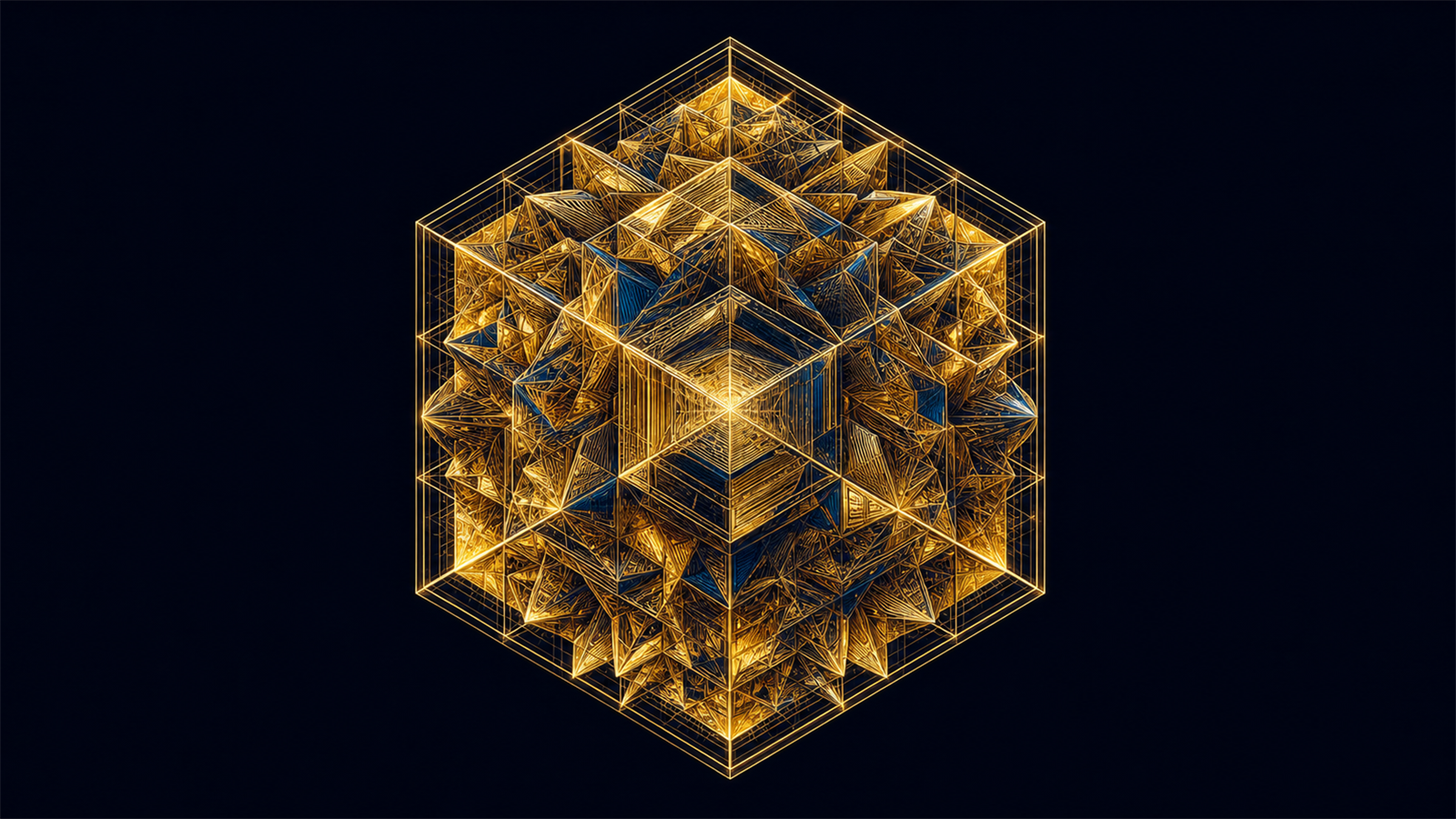 Figure · The Monster, as large as , has as the smallest space in which it can stretch its limbs only 196883 dimensions (): a colossal thing that fits exactly into its smallest room. (Made by this channel)
At this point the medical report is complete: size, fingerprint table, smallest home, all written, while the monster itself has not yet shown its face. In the next section, someone is going to really build it.
§3 · Building the monster by hand
By the end of the 1970s the situation was a little peculiar: all the technical data on the Monster (the order, the 194×194 character table, 196883, and even the 196884 about to come on stage below) was ready, but nobody had proved that it really existed. Conway later recalled his feeling at the time, saying that he regarded building the Monster as “a practical impossibility, or maybe an impractical possibility”.
 Robert Griess (1945–): in 1980, without using a single computer, he built the Monster by hand. (Photo by Renate Schmid, 2005, Oberwolfach Photo Collection, CC BY-SA 2.0 de.)
The one who broke this deadlock was Robert Griess. He was one of the first (around 1973) to produce evidence that the Monster exists. And he had in hand an extra clue passed to him by someone else: Norton deduced from that character table that the Monster must preserve a 196884-dimensional algebraic structure; that is, there is a “multiplication” on that 196884-dimensional space, and the Monster is exactly the full set of symmetries that do not scramble this multiplication.
This road sounds even harder than the original one: the thing to be built is bigger. But it is in fact easier: that group has elements, and you cannot write them down one by one; an algebra does not need to be written out one by one; giving a multiplication rule is enough. So the route was clear: first build this 196884-dimensional algebra, then prove that “the full set of symmetries preserving it” is exactly a new simple group, precisely the monster that had been predicted and whose medical report had already been written. On January 14, 1980, Griess announced in Ann Arbor: he had done it. Two years later the complete paper (titled The Friendly Giant, Invent. Math. 69) was printed, one hundred and two pages.
The most remarkable thing about this is that he did it by hand, without using a single computer. As a comparison: someone at the time did the arithmetic, and just doing one such matrix multiplication would take up a machine for seventeen or eighteen days: the matrices have nearly two hundred thousand rows and two hundred thousand columns, and by the most naive algorithm multiplications are needed; even at five billion per second, it would take seventeen or eighteen days. One multiplication, seventeen or eighteen days. And Griess completed the whole thing with paper and pen. Tits later said (in translation): “I simplified Griess’s construction slightly, but what he did is great work. It was done without a computer, which is a remarkable feat.” Griess himself recalled that he married in June 1979 and from October computed day and night without a break, “taking only half a day off for Thanksgiving and only one day for Christmas” (in translation).
A notation has to be made clear here, or experts can easily find fault: 196883 and 196884 differ by only , but refer to two things.
- 196883 is the dimension of the Monster’s representation: the smallest space in which it can stretch its limbs.
- 196884 is the dimension of that algebra. The usage current today calls this algebra the Griess algebra; the one dimension it has beyond the representation space is the direction of the algebra’s identity element (the "" that leaves anything unchanged when it multiplies it): .
(A point of historical precision: the algebra constructed in Griess’s original 1982 paper is in fact 196883-dimensional and contains no identity element; “adding a dimension for the identity to make 196884” is a cleaner later restatement. So one cannot say “Griess’s original paper constructed a 196884-dimensional algebra”. In this episode we use the current modern 196884 version, which is both correct and avoids this pitfall. For how the algebra is divided into blocks internally and where the multiplication comes from, see Appendix C.)
And the relation between the Monster and this algebra can be wrapped up with one equals sign. Here (automorphism group) is shorthand for “the full set of symmetries of some object”: all the transformations that keep this object’s structure exactly as it is, without the slightest disturbance, put together form a group. It runs completely parallel to the chain of equals signs in EP6:
The three objects in parentheses have all been seen with our own eyes earlier: is the Steiner design of EP6 ( points, points per block, any points lie in exactly one block), and is the full set of rearrangements that keep its block structure exactly as it is; is the Leech lattice of EP6 (the densest packing in dimensions, with kissing number ), and is the full set of orthogonal transformations preserving it; and the Griess algebra is exactly the -dimensional multiplication just built by hand in §3 of this episode, with the full set of symmetries that do not scramble this multiplication.
All along the way, the sporadic groups have each been “the full set of symmetries of some exceptionally intricate object”. The Monster is the largest one on this line.
The largest one in the box has at this point shown itself. But the extra "" on it () looks unimportant at the moment: its weight will only show in the last episode.
§4 · Twenty-six, and a proof that cannot be read to the end
With the Monster built, a very natural question pops up: is the box empty? Do the sporadic groups end here?
The count had in fact long since closed. The Monster and the several new subgroups it brought along pushed the total number of sporadic groups to 25; in 1975, Janko found evidence for the 26th (written ), and after that this number never changed again: 26 sporadic simple groups in all. In the previous episode we described how they split into families: of the 26, 20 are subgroups or quotient groups of the Monster, and the remaining 6 cannot be swallowed even by the Monster. And the one who named these two batches was exactly the person who built the Monster by hand: Griess, in The Friendly Giant, fixed both names in one sentence: the 20 that get in are called the “Happy Family”; those that do not, we already named in the previous episode: pariahs. His original words are:
“The sporadic groups which are involved in the Friendly Giant constitute the Happy Family and those which are not are called the Pariahs.” —Griess, The Friendly Giant, Invent. Math. 69 (1982), p. 3
But one detail is worth pausing on: in 1982 Griess could name only five pariahs (, , , , ); for the sixth, , he could not give an answer at the time. On the same page he wrote: “The membership of every sporadic group in one of those two categories is settled, except for ”, and added a very vivid remark: the order of is “only” 175,560, and “one might easily imagine a copy of floating as a tiny speck within ”.
In other words: the person who built the Monster by hand could not say for sure whether a small group of order one hundred seventy thousand was hidden inside the thing he had built. This suspense was only resolved in 1986 by Wilson (Robert Wilson), and the title of the paper is itself the question: “Is a subgroup of the Monster?” (Is a Subgroup of the Monster?, Bull. London Math. Soc. 18(4): 349–350, 1986, doi:10.1112/blms/18.4.349). The answer is no, and so the pariahs made up the full 6, becoming the number we write today.1
So, “has the classification of finite simple groups been completely finished?” The answer to this question brings out a theme that recurs in this series: a proof so long that nobody can read it to the end alone.
In 1983, Gorenstein (Daniel Gorenstein, 1923–1992) announced: the classification of finite simple groups has been fully completed. But this announcement came too early: he was misled by one proof into thinking that one class of cases, called “quasithin groups”, had been sealed, when in fact a gap remained there. Those who really filled this gap were Michael Aschbacher and Stephen Smith, and by then it was 2004: a proof in two large volumes totaling about 1221 pages. Only in that year was the classification of finite simple groups generally accepted as truly complete.
From Gorenstein’s proposal of the program in 1972 to the filling of the last piece in 2004, this classification project, which he himself called the “Thirty Years’ War”, spanned just about thirty years in all: that is exactly the theme of the EP5 episode. The appearance of the Monster (1980) falls in the middle of this war: it is the largest and also the most daunting item on this list that cannot be read to the end.
Epilogue · The box still has a crack
The Monster has shown itself. It is large beyond intuition (), yet it is an object that is finite, concrete, and can really be built by a pair of hands. It lives in 196883 dimensions, and its data has been checked again and again: and the people who checked it say themselves that the question of reliability has not gone away (see §2). It looks as if the story could wrap up here.
But one number will not keep still. The dimension of the Monster’s smallest representation is 196883, and the dimension of that algebra is 196884. And in a corner seemingly unrelated to group theory and to symmetry (a classical object in number theory called the -function), the first interesting coefficient of its expansion happens to be exactly 196884.
How can a number that describes the most space-saving form of the monster appear, without a digit’s difference, in a number-theory formula written down more than a hundred years earlier? Is it a coincidence, or is there one more thing hidden in the deepest part of the box?
The box still has one last crack. In the last episode we go and see what is behind that crack.
Appendix A (intuition + structure) · 3-transposition groups and mirror networks
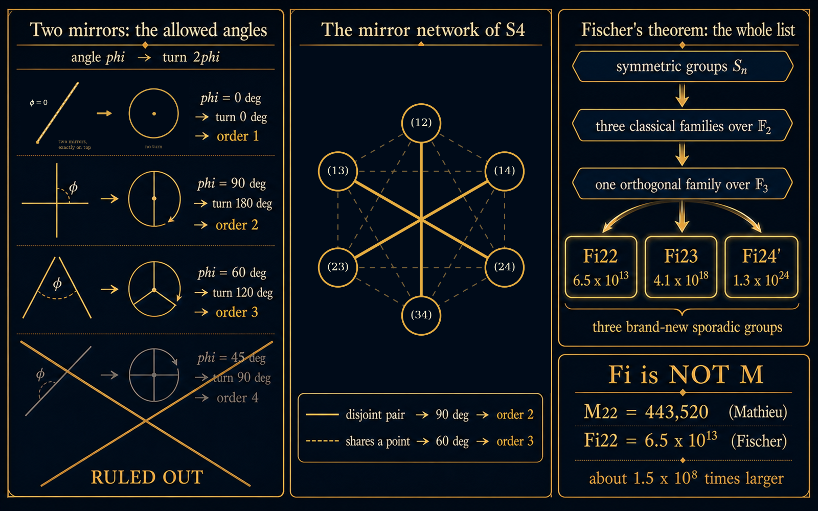 Figure A · Reflecting in two mirrors one after the other composes to a rotation, by twice the angle between them; so “the order of the product is at most 3” is the same as “the angle may only be coincidence, , ”, and is out. In the middle is the mirror network formed by the six transpositions of : the three solid lines are the only three pairs of disjoint transpositions (product of order 2), and the other twelve pairs all share a point (product of order 3). On the right are the three new sporadic groups that Fischer’s theorem closes on. The sign in the corner is the iron rule of notation: Fischer’s is not Mathieu’s . (Made by this channel · math infographic)
What this section does. Section §1 of the main text says that Fischer (Bernd Fischer), with the seemingly plain question of “groups generated by transpositions”, dug out three brand-new sporadic groups. Here we make “3-transposition group” precise, use the you know best as the instance, prove the statement “two mirrors compose to a rotation” that we have kept using as intuition, and then give the statement and intuition of Fischer’s theorem. The ceiling of this episode takes effect here: give the structure and examples; the complete classification proof is cited, not rebuilt.
Concept explained here: what is a 3-transposition group. A group generated by some conjugacy class (“conjugacy class” = a whole class of elements of the same type; EP4 Appendix 1 §2 gave the definition: the conjugacy class of = all ), where consists entirely of involutions (an involution returns to the identity after multiplying by itself once, : the entrance key drawn out of the odd order theorem in EP5 §3), and for any , the order of the product may only be , or . Such a is called a 3-transposition group. The three numbers each cover one case: order ; order the two involutions commute; order together they give rise to a small, triangle-like symmetry (we will see it with our own eyes in shortly).
Mirror intuition. An involution is like a mirror: reflecting twice = not reflecting. Reflecting in two mirrors in succession composes to a rotation, with angle = twice the angle between the two mirrors; so “the order of is ” translated into geometry is “the angle = ”. “Product order ” is therefore a rule for placing mirrors: any two mirrors either coincide, or meet at , or meet at , and no other angle is allowed. The whole group becomes a huge mirror network; what Fischer asked was: how many kinds of such networks can there be in all?
Below we set the two pillars of this intuition firmly in place one by one: first prove “two involutions always generate a dihedral group” (pure group theory, no mirrors needed), then prove “composing two mirrors = doubling the angle of rotation” (pure plane geometry), and finally put them together and see why that mirror-placing rule leaves exactly three angles.
Pillar one: any two involutions always generate a dihedral group (full proof).
Lemma. In a group , take any two involutions (that is, ). Write , . Then , and is the dihedral group of order , (the symmetry group of the regular -gon).
Proof. Since , , first compute the inverse: . Then compute the conjugate: that is, turns into its inverse. Also , so is generated by , and . The cyclic subgroup (of order ) is normalized by (the equation above), so , of order at most . When : if , then is commutative, and the equation above gives , , a contradiction; so , and the order is exactly . And , are precisely the defining relations of the dihedral group .
(: , and has order ; : commute, giving the Klein four-group: in EP5 §3, the involution centralizer in of order is exactly this. The two degenerate cases agree with the usual conventions for .)
This lemma is universal: “the order of is ” and ” generate the symmetry group of the regular -gon” are the same sentence. So “mirror” is not a figure of speech: the structure spanned by two involutions is, from the start, the symmetry group of a regular polygon.
Pillar two: composing two mirrors = a rotation, with angle = twice the angle between them (full proof).
For a line in the plane through the origin making with the -axis an angle , the matrix of reflection in it is
(Where it comes from: the unit vector making with the -axis an angle , , has a mirror image in this line that makes with the -axis an angle ; read , as the action of a matrix and you get it. You can check it on the spot: gives , which is exactly folding about the -axis; gives , which is exactly swapping the two coordinates along .)
Take two mirrors , , with angle between the two mirror lines. Multiply directly:
The four cells are, one by one, the angle-sum formulas: top left ; top right ; bottom left ; bottom right . The right-hand side is exactly the rotation matrix for angle .
Corollary: that mirror-placing rule leaves only three angles. A rotation by angle has order if and only if is times (in lowest terms), that is, the angle between the mirror lines is . Substituting one by one:
| Angle between the two mirrors | Composite rotation angle | Order of the product | Fischer’s rule |
|---|---|---|---|
| (coincide) | allowed () | ||
| allowed (the two mirrors are perpendicular, commute) | |||
| allowed | |||
| out |
Counterexample (). Two mirrors at compose to a rotation, of order , beyond . By the lemma of pillar one, these two involutions generate , of order , the symmetry group of the square. So: the symmetry network of the square as a whole cannot get onto Fischer’s list; the largest regular polygon that can get in is the equilateral triangle (, ). The mirror-placing rule “only coincidence / / ” is at this point no longer a convention, but all the values of for .
Honest boundary (an important point). The two pillars above have different strengths: the lemma is universal: in any group, any two involutions generate , without exception. The two-mirror theorem is plane geometry: it speaks about that geometric realization of . In a general 3-transposition group, is a conjugacy class of involutions, not necessarily actual mirrors in some plane (for example, for those families of classical groups over , “mirror” has to be understood in the geometry over a finite field; cited, not rebuilt). On the side, though, it holds literally: the transposition acting on is exactly the orthogonal reflection in the hyperplane (it fixes that hyperplane and reverses the sign of ); in the instance below, the two methods of computation will match on the same answer.
Instance: itself is a 3-transposition group. Take all transpositions (swap two points, leave the rest unmoved; cycle notation was just learned in EP6 Appendix B). Taking any two transpositions, there are exhaustively only three possible relative positions:
- Equal: , order .
- Disjoint: : each moves its own points without interfering, they commute, and the product has order .
- Sharing one point: , a -cycle, order .
There is no fourth case, so the product order is always : is a 3-transposition group (checked by enumerating pair by pair over the transpositions of , all of them, without exception).
The two roads match. Recompute the three lines above with mirrors: the mirror of the transposition is the hyperplane , whose normal vector (the “root”) is ; the angle between two mirrors = the angle between the two roots. For the disjoint , the roots and are orthogonal, the angle is → rotation angle → order . For sharing a point, the angle between the roots and is given by as → rotation angle → order . Line by line in agreement with the orders obtained by counting cycles directly (both methods went into the check). is the smallest nontrivial mirror network: three mirrors, pairwise at .
Fischer’s theorem (1971, cited at the level of statement). Under technical hypotheses of the kind “no nontrivial solvable normal subgroup”, the list of finite 3-transposition groups is abnormally short: the symmetric groups ; three families of classical groups over (symplectic groups , unitary groups , orthogonal groups , all on the “Lie-type families” list of EP5 §1, of which the unitary groups were constructed explicitly in EP5 Appendix D); one family of orthogonal-type groups over ; and exactly three new groups that nobody had seen before: , , . The iron rule of notation struck once more (the mine planted in the EP6 epilogue): Fischer’s and Mathieu’s are two different families: , about one hundred fifty million times larger than . . itself is not simple: it contains a normal subgroup taking up exactly half of it (the bookkeeping of Lagrange’s theorem in EP2 group theory mini-lesson ④: index ), and it is that half that is the sporadic simple group, written (the prime is the mark for “take that half”), . All three orders checked against the ATLAS (the products have been computed). The complete proof of the theorem belongs to Fischer’s original paper “Finite groups generated by 3-transpositions. I” (Invent. Math. 13 (1971) 232–246), cited, not rebuilt.
From to : the ramp to the Monster (details of the historical line belong to main text §1–§2). Loosen the mirror-placing rule by one notch, allowing product orders up to (so-called -transposition groups; by the table above, this is exactly letting in), and push the same mirror-network philosophy further: along this ramp Fischer first touched the Baby Monster ; and the prediction of the Monster (around 1973, proposed independently by Fischer and Griess (Robert Griess)) was exactly “there exists a simple group in which the centralizer of some involution contains a double cover of ” (“double cover” = a shelled version exactly twice as large as the original group, which goes back to it after quotienting out the center : in EP6, stands in exactly this relation to ). The involution centralizer, that knife of local analysis from EP5 §3, is drawn from its sheath for the third time.
Symbolic check: the transpositions of , all , enumerated pair by pair ( pairs), product order always , and “equal / disjoint / sharing a point ” holds pair by pair; on the same pairs holds pair by pair (dihedral lemma); has order ; the two-mirror theorem fully proved as a symbolic identity ( equal cell by cell to the rotation matrix for angle , not a numerical approximation), and , ; cross-check of the mirror realization: root angles agree line by line with permutation product orders ; the product of two mirrors at has order and generates (order ); the products of prime factors for the three Fischer group orders agree digit by digit with the decimal integers (against the ATLAS); . The list in Fischer’s theorem itself = citation (the 1971 original), not part of the check.
Appendix B (intuition + structure) · The character table and 196883
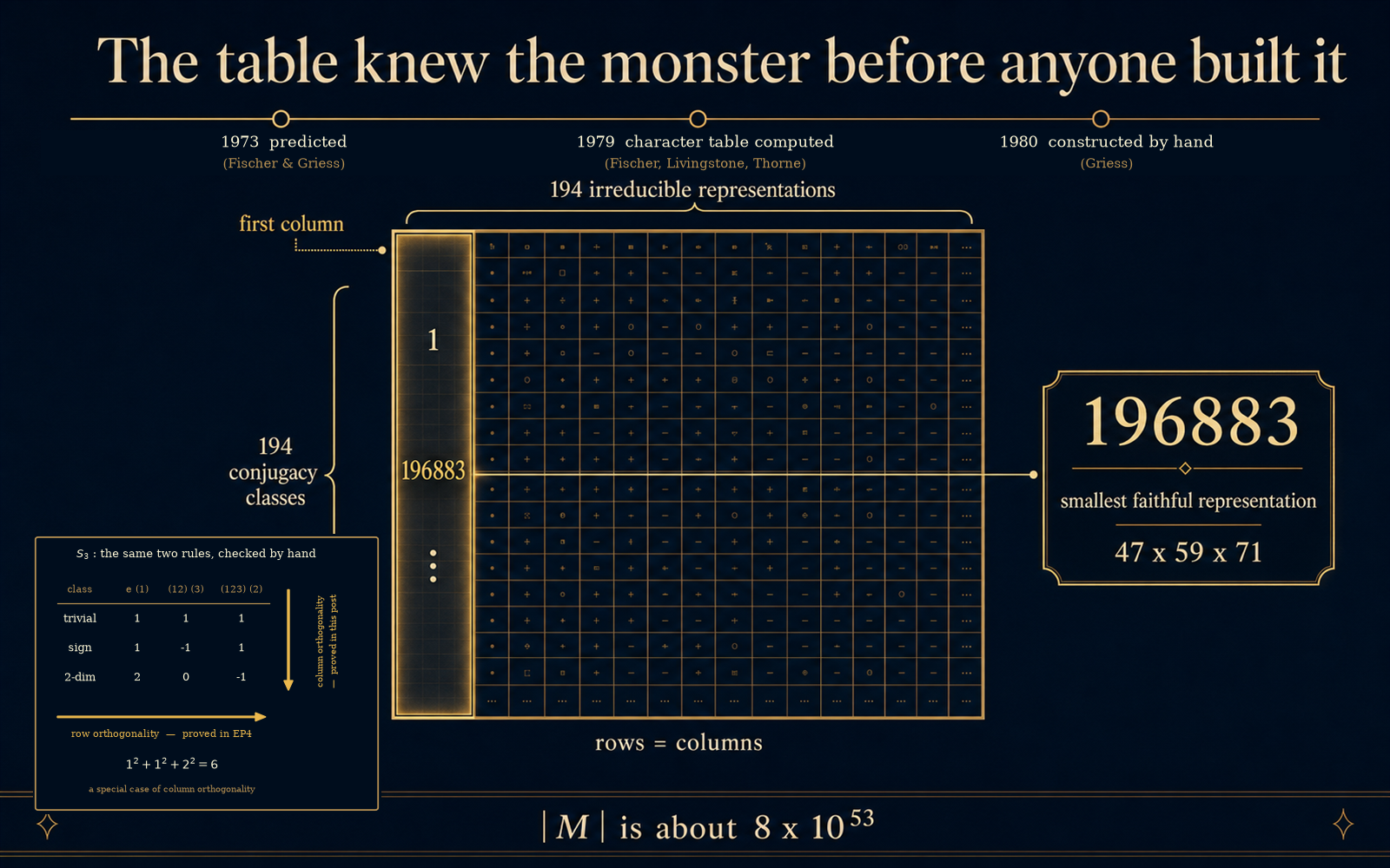 Figure B · The character table of the Monster: the number of irreducible complex representations = the number of conjugacy classes, so this table must be square: 194 across and 194 down. The first column lists the dimension of each representation; at the top is , and immediately after it, the second, is (the three largest prime factors in the Monster’s order). The lower left corner uses ‘s small table to lay out the same two rules and compute them: row orthogonality was already proved in EP4 Appendix 1, column orthogonality is the one added in this episode, and is just its special case on the first column. The timeline at the top is the crux of this episode: 1973 prediction, 1979 table finished, and only in 1980 did someone build it. (Made by this channel · math infographic)
What this section does. Section §2 of the main text says the Monster’s “medical report” existed before the Monster itself: the character table had been computed by 1979, while the group would only be built in 1980. Here we make clear: what a character is (the four words planted in EP4 become regular here), how this table is read, which cell of the table stands in, and on what grounds “computing a group’s table without having seen the group” is possible. This section is the engine of this episode’s core claim, so it is one notch harder than elsewhere: the theorem that makes the whole thing hold (the table must be square), together with the column orthogonality relation, is proved all the way here (EP4 Appendix 1 only proved the row half). The Monster’s table itself is cited from the ATLAS, not recomputed.
Concepts explained here (calling back to EP4). These four words were given in full, with definitions and proofs, in EP4 Appendix 1 (“Foundations of representation theory: complete reducibility, characters, Schur orthogonality”); here we wake them up and reuse them: representation (faithfully translating group elements into matrices, , with the multiplication structure preserved), dimension (the size of the matrices), irreducible (the smallest blocks that cannot be broken down: any representation can be broken into a platter of irreducible blocks, the complete reducibility of EP4 Appendix 1 §1), character (, the sum of the diagonal entries of the matrix, the “fingerprint” of a representation). A key convenience: the trace does not move under change of basis, so elements in the same conjugacy class have the same fingerprint: a character only needs one number recorded per class (such a function is called a class function: a function taking a constant value on each conjugacy class).
Arranging them in a square matrix gives the character table: rows = irreducible representations, columns = conjugacy classes, and cell = the trace of the -th irreducible representation on the -th class. The first column (the column of the identity element) is exactly the dimensions of the representations, because .
And “number of rows = number of columns” (the number of irreducible complex representations is exactly equal to the number of conjugacy classes) is not a coincidence of notation but a theorem. (The word “complex” cannot be dropped: over the real numbers, or when the characteristic divides , this equality no longer holds. Wherever the text below and the figures simplify, complex representations are meant throughout.) It is the foundation of this episode’s statement “computing a group’s table without having seen the group”, and we prove it below.
Waking up: the table of EP4 Appendix 1 §3. (the symmetry group of the equilateral triangle dissected throughout the group theory mini-lessons of EP2) has conjugacy classes: , the three transpositions, the two three-cycles, of sizes respectively; it has exactly irreducible representations, whose characters are written (trivial), (sign), (standard two-dimensional). The whole table, together with the term-by-term check of row orthogonality, was already done in EP4 Appendix 1 §3; we do not re-derive it here, but just take the three rows of values as raw material for what follows:
(The three columns correspond in order to the classes , transpositions, three-cycles, with class sizes .) What EP4 checked on this table was the orthogonality of row against row; what this section is to prove is that column against column is orthogonal too: the same table, turned sideways and used once more.
Theorem 1: the table must be square (full proof).
Theorem. For a finite group , the number of irreducible complex representations (up to isomorphism), , is exactly equal to the number of conjugacy classes of , .
Proof. Write = the complex vector space formed by all class functions on , with the inner product carried over from EP4 Appendix 1 §3, . In three steps.
Step 1: . A class function takes one constant value on each conjugacy class, and these constant values can be specified arbitrarily; so take the indicator functions of the classes (on taking , elsewhere ); they are clearly linearly independent and span . Hence .
Step 2: . EP4 Appendix 1 §3 already proved the first orthogonality relation : the irreducible characters are a set of orthonormal vectors in , and therefore linearly independent. An orthogonal set in a -dimensional space has no more than members, so .
Step 3: they also span , so . It suffices to prove: if is orthogonal to every , then (orthogonal complement is zero spanning). Suppose for all . For each irreducible representation , construct the operator
It is an intertwining operator: for any ,
where the change of variable in the middle step is a bijection from to itself, and the last step is exactly where we use that is a class function (). Hence .
By Schur’s lemma (b) (already proved in EP4 Appendix 1 §3), . Take the trace to determine : so , that is, : this holds for every irreducible representation.
Then by complete reducibility (already proved in EP4 Appendix 1 §1): any representation is a direct sum of irreducible representations, and the construction of proceeds block by block on a direct sum, so for any representation we have . In particular take the regular representation (the one used when counting multiplicities at the end of EP4 Appendix 1 §3: with the group elements as basis , ), and apply this zero operator to the basis vector :
And is a basis, so the coefficients must be zero one by one: for all , that is, .
So the irreducible characters are an orthonormal basis of , and . The character table is a square matrix: as many conjugacy classes as there are, so many irreducible representations there are, not one more, not one fewer.
Theorem 2: the column orthogonality relation (full proof).
Theorem (second orthogonality relation). For , where = the subgroup consisting of all group elements that commute with (the centralizer).
Proof. By Theorem 1, the irreducible representations and the conjugacy classes both number , so the whole table can be packed into a square matrix :
First look at ( = conjugate transpose): (in the middle, “summing by class, multiplying by class size” is restored to “summing over group elements”, because a character takes a constant value on each class). What this step uses is exactly the row orthogonality of EP4 Appendix 1 §3. So
The key step is here: is a square matrix, so means , and therefore the other side holds too: Write it out:
Read it in two cases:
- (different classes): the right-hand side , and the coefficient in front is nonzero, so .
- (same class): , that is, . And by the orbit–stabilizer theorem (walked through explicitly in EP5 Appendix H to compute ‘s ), let act on itself by conjugation: the orbit of is exactly its conjugacy class , and the stabilizer is exactly its centralizer , so .
Why the square-matrix step cannot be skipped. “Row orthogonality implies column orthogonality” relies entirely on being a square matrix: for a non-square matrix, does not imply . A example is enough to see it: take ; then (the “row” is orthonormal), but So Theorem 1 (the table is square) is not a polite preliminary to Theorem 2; it is the pile cap on which Theorem 2 stands. This is also where the real weight of the statement ” conjugacy classes the table is ” lies.
Verifying column orthogonality on (the three rows of values woken up earlier, used sideways). First compute the centralizers: of order ; of order ; of order . (One can also use directly: ; they match.)
- Same column (the sum of squares of the column the order of the centralizer of that class):
- Different columns (pairwise zero):
Collecting along the way an iron law that previously we only copied down. Look at the first formula above: the sum of squares of the column . This is not a coincidence: apply column orthogonality to the column of the identity element (): , and , so
“Sum of squares of the dimensions = order of the group” is the special case of column orthogonality on the first column. Elsewhere it is often treated as a formula to memorize; here it is proved.
The Monster’s table: a “medical report” that came before the group itself. After the ramp at the end of Appendix A led to the prediction around 1973, what mathematicians had in hand were only assumptions: assume exists, assume the centralizers of its two classes of involutions look like that (one class tied to the double cover of the Baby Monster, the other : the of EP6 comes back on stage here; reads as “wearing a binary shell of layers”, and it grows exactly around the Leech lattice). On the strength of these assumptions plus the iron laws of character theory alone, the order was determined by working backward:
( decimal digits: ; the product has been computed). In the 1970s (finalized by 1979; for the discrepancy in years across three sources see §2), Fischer and Livingstone (Donald Livingstone), with the help of a program written by Thorne (Michael Thorne), finished computing the whole character table: at this point the Monster had still not been proved to exist. One more is missing: the dimension divides the order of the group (short, using the algebraic-integer toolbox). Besides the three constraints above, one more was used again and again in working back to the character table: the dimension of each irreducible representation divides . It comes easily: EP4 Appendix 5 §1 already proved that the central character is an algebraic integer, and from row orthogonality , grouping by class and dividing by :
The right-hand side is an algebraic integer ( and are both algebraic integers, and the algebraic integers form a ring); the left-hand side is a rational number. And the algebraic integers in are exactly , so is an integer, that is, . (Here “the algebraic integers form a ring” and “the algebraic integers in ” are number-theoretic background, borrowed from EP4 Appendix 5 §0 and throughout this series cited, not rebuilt: re-proving them belongs to algebraic number theory and is not within this episode’s ceiling.)
On what grounds it is possible. Now we can answer head-on the statement in main text §2, “the medical report came before the thing itself”. With only a few assumptions about involution centralizers in hand, it was enough to force a table to be almost unique, relying on these constraints just proved, which bite into each other:
- The table is square (Theorem 1): conjugacy classes means there must be irreducible representations, not a single cell more;
- Rows are orthonormal to each other (EP4 Appendix 1 §3);
- Columns are orthogonal to each other, and each column’s sum of squares the order of the centralizer of that class (Theorem 2): the orders of the centralizers are exactly the quantities those assumptions give directly, so the assumptions turn directly into numerical constraints on the table;
- (the special case of Theorem 2 on the first column) and : these pin the sequence of dimensions into a very narrow range.
How tight are these conditions: they do not “help” determine this table; they almost lock it in. What that machine did in 1979 was fill in the cells one by one under these constraints: what it filled in was the medical report of a monster that at the time nobody had seen, and that had not even been proved to exist.
There is one more machine: computing the order directly. The four constraints above force the table into a very narrow space; but the number itself was given by another tool, the Thompson order formula (main text §2 said what it takes in and what it puts out; here we give its shape): suppose has exactly two classes of involutions, with representatives , ; then
where counts those involution pairings ( conjugate to , conjugate to ) in which falls inside . By the dihedral lemma of Appendix A, is a dihedral group and is exactly its rotation half: so what counts is “in the rotation part of which dihedral blocks can be seen”. The Monster has exactly “two classes of involutions” (2A, 2B), so the premise fits exactly. And so the whole chain closes: assumptions ⟹ two neighbor circles ⟹ order ⟹ combined with the orthogonality relations ⟹ the whole , all without ever having seen that group. (For the complete proof of the formula see Appendix D: it is cheaper than any passage of this appendix: it needs only that dihedral lemma of Appendix A plus one double count, and does not touch characters.)
Where is. Look at the first column of the table (the dimensions of the irreducible representations): at the top is always (the trivial representation); for the Monster, the second-smallest dimension is exactly : it is the smallest dimension of a faithful complex representation of (“faithful” = different group elements correspond to different matrices, explained in EP6 Appendix D; the trivial representation maps everything to , the least faithful). Moreover
is exactly the product of the three largest in the list of prime factors of (computed). A colossus of needs, even for its most frugal matrix home, dimensions. (A note on the convention: this is the answer over the complex field , the ATLAS convention; change the field and the number moves: for example over the smallest faithful dimension is ; we only touch on this.)
A small piece of the real table. The whole cannot be printed here (in the ATLAS it takes up several pages, and the cells hold algebraic integers). But the first column (the dimensions of the irreducible representations) can be glanced at. The first ten entries, in ATLAS order:
Three things are worth making clear with these ten numbers.
One: dimensions, not “different” dimensions. We proved above that “number of irreducibles = number of conjugacy classes”, so this column has exactly entries, no more and no fewer; but only of them are mutually different: some dimensions are shared by two different irreducible representations (the th and th entries, for example, are both ), and in one place three share one. Same dimension does not mean same representation: they can be told apart in the other columns. This is exactly why the character table has to have columns: looking only at the first column is not enough.
Two: every dimension divides . The statement above can be checked entry by entry here: these ten entries (and indeed all ) without exception. This is not a coincidence but a direct consequence of that theorem; back when this table was worked out backward, it was exactly one of the sieves used to filter out candidate dimensions. (A word of caution on proportion: divisibility is only a necessary condition; it can filter out the wrong ones but cannot sift out the right one: it can falsify, it cannot endorse.)
Three: the first four entries can be matched independently with the j-function. The coefficients of the j-function are defined by , have nothing whatsoever to do with the Monster, and can be computed completely independently: , , . Match them against the dimensions above:
The three lines fit perfectly. This means the first four dimensions above are not “copied”: they have been independently checked once by a set of numbers from a completely unrelated source. As for why the coefficients of j are “exactly” sums of these dimensions: here we only lay out the arithmetic; that “why” is the business of the last episode. (This independent corroboration goes only up to the fourth entry; from the fifth entry on there is no such handle, and we can only cite the ATLAS.)
Four: this table was recomputed in 2024. First, one thing that is easily skipped over: the derivation of that original computation was never publicly published; Wilson himself recalled (in a December 2024 blog post) that “the calculations were so long and complicated, that nothing was ever published”. That is to say, for this table, cited over and over for more than forty years, the working draft was never in the public record.
As part of a project to “recompute all the character tables in the ATLAS”,
Breuer (Thomas Breuer), Magaard (Kay Magaard) and Wilson (Robert Wilson) redid the Monster’s table (arXiv:2412.12182). Their starting point is worth mentioning: under the assumption of the Monster’s uniqueness, plus the premise that “there exists a -dimensional faithful representation”, they determined all the conjugacy classes and the orders of the centralizers: the same machine as in (exactly the column orthogonality proved above: the sum of squares of each column is exactly equal to the order of the centralizer of that class). Forty-five years on, walking the same set of constraints once more, it still goes through. And what they wrote at the start of the paper is:
“The table was checked in various ways before publication in the ATLAS in 1985, and its incorporation into GAP. Nevertheless, the problem of reliability and reproducibility of this table remains.”
Among the people who wrote this, Wilson is one of the five editors of the ATLAS, and Breuer is the author of the GAP character table library, that is, the library where this table is stored today. The people who compiled it back then and the people who keep it today, forty-five years later, looked back together to re-verify it, and said that the problem of reproducibility still exists. This is exactly another face of that EP5 motif: some things are too big to be verified completely by one pair of hands.
(Source of the dimensions: OEIS A001379 “Degrees of irreducible representations of Monster group M”: the data is generated by GAP’s CharacterTable("M") and originates in the ATLAS; the complete entries are in that entry’s b-file; entries / distinct, and the repetition in entries –, also come from that entry’s notes. The arithmetic of the three moonshine identities above, and “each entry divides ”, have been computed entry by entry for this episode.)
Why keep an eye on it (the hook to EP8). The epilogue of the main text says that the coefficient of the j-function is : off by exactly a . What is that ? Appendix C gives it a concrete identity right away.
Symbolic check: the table: first column = dimensions, , all pairs of rows weighted-orthogonal (including norm ), all pairs of columns orthogonal and the sum of squares within a column equal column by column to the order of the centralizer of that class, (and checked independently against ), ; the counterexample to squareness (the satisfies while , checked cell by cell); the product of the prime factors of agrees digit by digit with the -digit decimal (against the ATLAS); ; the three largest in the set of prime factors of are exactly ; . The proofs of Theorem 1 / Theorem 2 / are proofs in words ( checked as their instance). That small piece of the real table: the -expansion of the j-function is computed from scratch from (an exact integer series), giving , , ; the dimensions are cited from OEIS A001379 (its generated by GAP
CharacterTable("M"), its pointing to ATLAS 1985); the three moonshine identities collide the computed j-coefficients with the cited dimensions, all equal ⟹ independent corroboration of the first four entries (only the first four entries; from the fifth on, cite-only). The first entries each divide : necessary, not sufficient, not taken as an endorsement. The repeated entry occurs twice among the first entries (against the note’s entries / distinct). The Thompson order formula step: ( taken from EP6, already checked within the series); it divides (Lagrange, a real test); digit count vs ‘s , exactly half, the same order of magnitude as . The formula itself, the definition of , the classes and the centralizer structure of 2A/2B, the sequence of dimensions, and ‘s = cited (Thompson’s original work / ATLAS / Breuer–Magaard–Wilson), not part of the check.
Appendix C (structural skeleton) · The Griess algebra
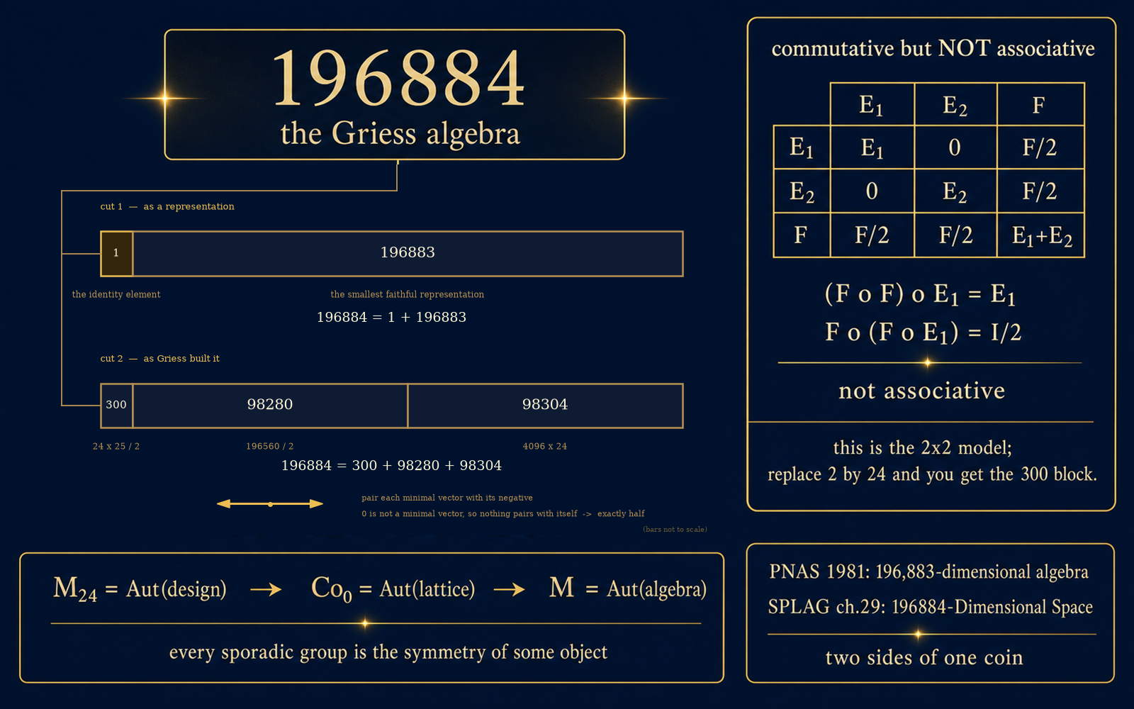 Figure C · The Griess algebra. The dimensions are cut twice, and both cuts cut the same ; it is not one cut nested inside another. The first cut is by representation: (the one dimension spanned by the identity element) + (the smallest faithful representation): the identity of what lies between and , that , is right here. The second cut is the block division Griess actually used when building it: (all symmetric matrices on the -dimensional Leech space, ) + (the minimal vectors of EP6, paired off as and halved) + (). On the right, the whole multiplication table of the small model is computed out: commutative, with identity element , but not associative; replace by and you get that block. (Made by this channel · math infographic)
What this section does. On January 14, 1980, Griess announced: he had built the Monster without a computer, by hand. The method was first to build a -dimensional algebra, then prove that “the full set of symmetries preserving this algebra” is exactly a new simple group, precisely the monster that had been predicted and whose medical report had already been written in advance. Here we give the skeleton of the construction: how is divided into blocks, where the multiplication comes from, and what “the Monster ” means. In two places we are not content with “reporting numbers” and make it computable by hand: the multiplication of the block is laid out as a full table on a three-dimensional small model, and the “halving” of is given a proof that the pairing is well defined. The cross-block multiplication and the correctness of the construction remain at the structural level: the hundred pages of verification in Griess’s original paper are cited, not rebuilt (Griess 1981/1982, Conway 1985, SPLAG Chapter 29).
Concept explained here: algebra. A vector space, equipped in addition with a “multiplication” (bilinear: linear in each factor). Commutative = ; associative = . Matrix multiplication is associative but not commutative; what is wanted here is exactly the opposite: commutative, but not associative. The prototype is symmetric matrices with the Jordan product
(multiply once in each direction and take the average; when are symmetric the result is still symmetric). Commutativity holds unconditionally (swapping in the defining formula leaves it unchanged); associativity in general fails. Below we lay this out as a full table in a three-dimensional small model: it is a miniature version of the block.
A small model of the block: replace by (full table computable by hand). The dimension of symmetric matrices is ; taking gives , exactly that block; taking gives : three-dimensional, small enough to write out the whole multiplication table. Take as basis
Compute cell by cell (each cell is two matrix multiplications followed by an average; you can recheck it yourself): , so ; likewise ; , so ; , so ; , , adding the two gives , so ; likewise . The whole table:
The table is symmetric along the diagonal: commutative, visibly. The identity element is : , ; each basis element is unchanged. And the failure of associativity can be computed from the table:
: the same three elements; change where the parentheses go and the answer changes. (Exact fractions computed.) “Commutative, non-associative” is not pathological: it forms a kingdom of its own (Jordan algebras, the algebra of observables in quantum mechanics), and the Griess algebra lives next door to it.
Change back to , and this table grows unchanged into that -dimensional block: likewise commutative, likewise with identity element , likewise not associative. (The block, under the action of , further splits into , and that is the direction spanned by : cited from Conway 1985 / SPLAG Chapter 29, not rebuilt.)
The two splittings of . The first cut (as an -module: “how it breaks apart under the Monster’s symmetry”):
The dimension = the direction spanned by the identity element (the “unit” of the algebra: anything multiplied by it is unchanged; the in the small model above plays exactly this role); the dimensions = that smallest faithful representation of Appendix B. This is the concrete identity of what lies between and , that . The second cut (the one used during the construction; at that time there was no yet, only the “known local symmetry” in hand, and the division into blocks follows it; the whole Leech chain of EP6 returns):
- = all symmetric matrices on the -dimensional Leech space (dimension ): the multiplication prototype is exactly the table above.
- = the minimal vectors of EP6, paired as and halved, one basis direction per pair. The kissing number of EP6 comes back to life unchanged inside the Monster. (This “halving” is proved below.)
- = : the shell group comes with a -dimensional representation of its own (: again the number of Golay codewords, EP6 Appendix B), paired with the dimensions. (To avoid confusion: also appeared in EP6 Appendix C when counting minimal vectors; there it was the number of vectors of the class “one plus twenty-three ” (); the here is the dimension of a block. The same arithmetic, two different things.)
That “halving” is not a casual division (full proof).
Proposition. Let = the set of minimal vectors of the Leech lattice , . Then partitions into pairs , every one of them with two elements, and the number of pairs is exactly .
Proof. Write .
(i) maps to . A lattice is an additive group, ; also , the norm is unchanged, so minimality is preserved.
(ii) is an involution. .
(iii) has no fixed points on : this step is the whole crux. , which in the real vector space happens only for . And : the norm of a minimal vector is (the scaling convention of EP6 Appendix C: the integer representatives have norm , which, multiplied by , gives ), while . So no vector in is paired with itself.
(iv) Counting. A fixed-point-free involution partitions into orbits each containing exactly elements (the orbit , whose two elements are distinct by (iii)). So must be even, and the number of pairs .
Why this step is worth writing out. The halving does not rely on “dividing by is always right”, but on that sentence in (iii): is not among the minimal vectors. If even a single self-paired element () got mixed into the set, an orbit with only element would appear, would immediately no longer be the number of pairs, and the dimension would not stand. The three classes into which EP6 Appendix C split each bear this out class by class: each class is closed under negation, and each count is even:
(Halving the three classes one by one and then adding matches halving the total: part of the check.)
Where the multiplication comes from. Each of the three blocks has a natural multiplication prototype (the Jordan product for the symmetric-matrix block, the geometry of the lattice for the minimal-vector block, the algebra of the code for the block); the real difficulty lies in how to fill in the cross-block multiplication table, filling it so that the symmetry group of the whole is strictly larger than the visible to the naked eye. Griess tuned that cross-block multiplication table by hand, and then proved that its full set of symmetries forms exactly a new simple group. “Beyond the visible symmetries, there are extra symmetries coming in at a slant”: the motif of that third class of “slanted” elements of in EP6 Appendix D replays unchanged one level up.
The Monster . = this -dimensional commutative non-associative algebra (in modern usage generally called the Griess algebra):
: all linear transformations preserving the multiplication (together with the accompanying inner product) (the notation reads “the group formed by all automorphisms of ”, that is, all structure-preserving rearrangements of ; explained in EP6 Appendix A at ). A column of equals signs completely parallel to EP6 wraps up the motif of the whole series: , , : the sporadic groups have all along been “the full set of symmetries of some exceptionally intricate object”.
or ? Two sides of one coin (a note on notation). The title of Griess’s 1981 PNAS announcement says in black and white “…automorphisms of a 196,883-dimensional algebra” (his original algebra has no identity element); the Griess algebra in modern usage is taken as -dimensional (adding the identity direction ): the title of SPLAG Chapter 29 is “The Monster Group and its 196884-Dimensional Space”. Two packagings of the same thing; at the j-function end of EP8, what is waiting is .
Wrapping up. The character table is an a priori blueprint: those orthogonality relations of Appendix B guarantee that it can be filled in before the group is built; Griess’s algebra was the first time the building on the blueprint was really put up. Tits (Jacques Tits) and Conway then greatly simplified the construction (Conway 1985; SPLAG Chapter 29 is its readable version). The largest one in the box has shown itself.
Symbolic check: , (dimension of the small model); ; ; ; ; the three-dimensional Jordan small model’s full table of nine cells checked cell by cell (including , , ), commutativity checked cell by cell, the identity element checked against each of the three basis elements, (exact fractions); ; the class-by-class evenness of the three classes of and the sum of halves (against the of EP6 Appendix C, with the sum of the three classes checked independently). The module structure of the blocks, , the cross-block multiplication, = cited from Griess/Conway/SPLAG, not rebuilt.
Appendix D (full proof) · The Thompson order formula
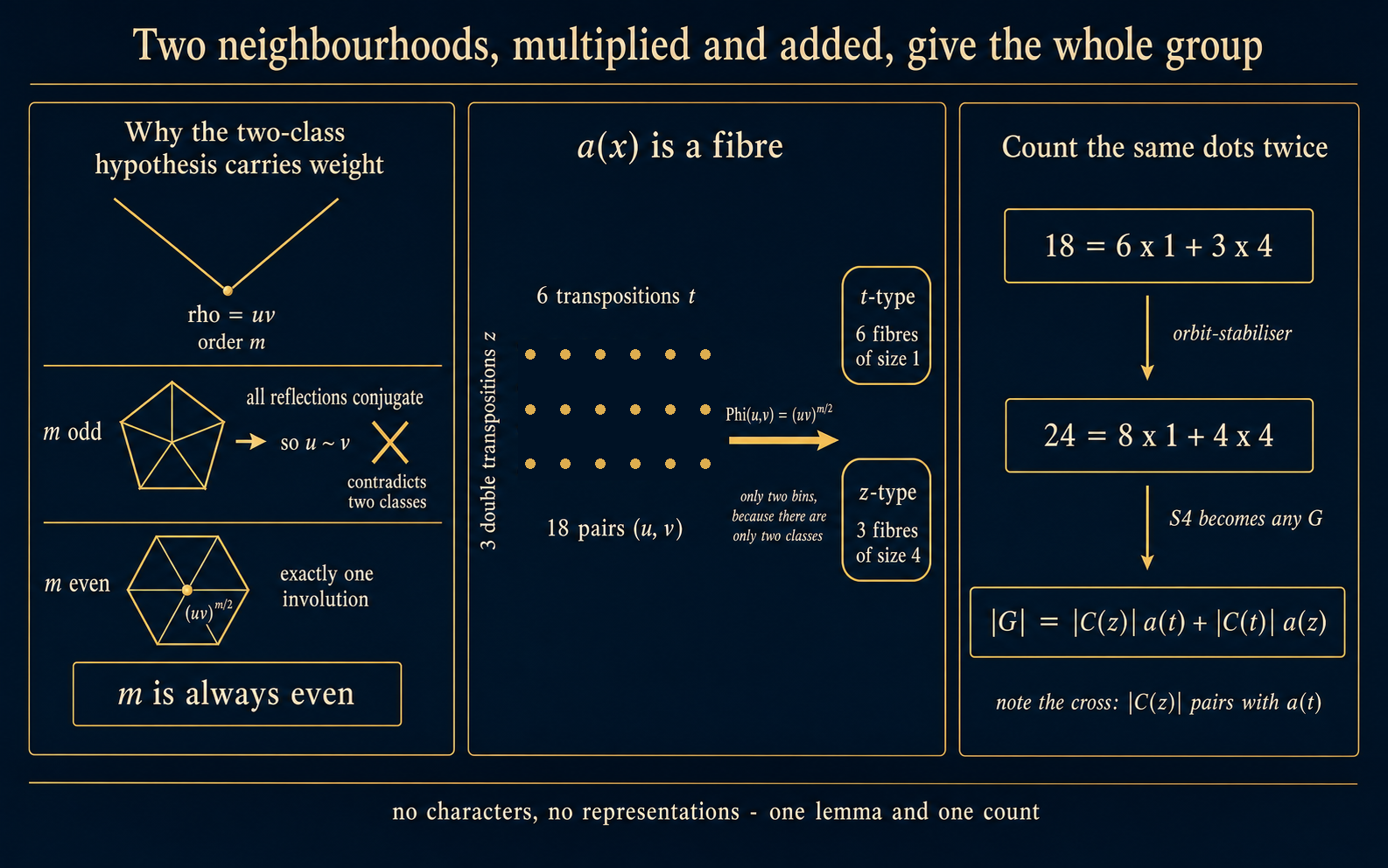 Figure D · The Thompson order formula. Left: why the premise “exactly two classes of involutions” carries load: if the order of the product of two mirrors is odd, all reflections in are conjugate to each other, so , contradicting “two classes”; so must be even, and even guarantees that the cyclic group contains exactly one involution . Middle: this uniqueness turns into a fiber of a map : in the figure, ‘s pairings are sorted by into only two buckets (because there are only two classes of involutions). Right: count the same set of points twice: ; after substituting orbit–stabilizer, , and replacing by an arbitrary gives that formula. That crossing ( paired with ) is a leftover of bringing to a common denominator, not a convention.
What this section does. Main text §2 said that the Thompson order formula “takes in the neighbor circle of an involution and puts out the order of the whole group”, and hung it up as a citation. Here we prove it, and the reason for doing so is that it is cheaper than any other passage of this article:
No characters needed, no representation theory needed, none of Griess’s hundred pages needed. All the equipment is that dihedral lemma of Appendix A, plus one double count. For scale: in Appendix B, “number of irreducibles = number of conjugacy classes” used Schur’s lemma and the regular representation, and column orthogonality used a squareness argument: the Thompson order formula is shallower than both of these. It looks deep because the [conclusion] is astonishing, not because the [proof] is hard. The first time the Monster’s order was written down, it relied not on some new machine but on a count an undergraduate can follow. What was hard was always daring to guess that it exists.
1 The theorem
Theorem (Thompson order formula). Suppose the finite group has exactly two conjugacy classes of involutions, with representatives , . For define Then
Notation: is the conjugacy class of (defined in EP4 Appendix 1 §2); is the centralizer; denotes the order. Involution = and (that entrance key from EP5 §3).
⚠️ Note the crossing: is paired with , not with . This is not a slip of the pen; in §5 below we will see that it grows out of the algebra itself.
2 The premise carries load; it is not decoration
The condition “exactly two classes of involutions” is really used in the proof, and in the most crucial step. It guarantees:
(Two different conjugacy classes are disjoint.) The pivot of the whole proof is this “not conjugate”: Lemma 3 of §3 relies entirely on it.
The Monster qualifies exactly: has exactly two classes of involutions, written 2A and 2B in the ATLAS. The premise fits; it is not contrived.
3 The chain of lemmas
Lemma 1 (dihedral lemma): already fully proved in Appendix A §Pillar one; here we only cite ourselves
In a group , take any two involutions . Write , . Then , and is the dihedral group of order , , in which is exactly the “rotation” half (the cyclic subgroup of index 2), and both fall in the “reflection” half.
(Proof in Appendix A; already checked by enumeration on all 225 pairs in .)
Lemma 2 ( odd all reflections in one class)
(, a reflection). If is odd, then all reflections are already conjugate to each other inside .
Proof. The reflections are exactly (). Conjugate by rotations: (Since , we have ; then multiply on the left by .) odd is invertible in as runs over , also runs over all reflections are in the same orbit.
When is even the reflections split into two classes ( odd / even), because runs only over the even numbers. This odd/even difference is the entire content of the next lemma.
Lemma 3 (the key: must be even)
, is even.
Proof. By contradiction. Suppose is odd. By Lemma 1, , and are both reflections in it. By Lemma 2 ( odd), are conjugate within , and hence conjugate in . But and belong to two different conjugacy classes and cannot be conjugate. Contradiction.
The premise is cashed in here: if had only one class of involutions, would not be a contradiction, this step would collapse immediately, and the whole formula would not hold.
Lemma 4 (unique involution)
even the cyclic group (of order ) contains exactly one involution, namely .
Proof. In a cyclic group, the subgroup of each order dividing the group’s order is unique, so the subgroup of order 2 is unique, so the involution is unique. even guarantees that it exists.
Corollary (the pairing map is well defined)
By Lemmas 3 + 4, one can define where is all the involutions of (premise: only two classes).
And for an involution : ( is obvious; follows from the uniqueness in Lemma 4). Hence
This is the turning point of the whole proof: goes from a “count that looks very strange” to a fiber of a map. And fibers partition the domain: that is the entrance to the double count.
Lemma 5 ( is a class function)
for all .
Proof. is a bijection from to itself (conjugacy classes are closed under conjugation). Also , so , and hence This bijection maps bijectively onto .
4 The double count (the true form of the main text’s “multiply once, add once”)
The fibers of partition the domain (each pair falls into exactly one fiber):
How to read it (can be given directly to the audience): lay out all the pairings “one involution of type with one involution of type ”. Each pair generates a dihedral block; in the very middle of each block sits exactly one involution (Lemma 4). So sort the pairings into piles by “who is the one in the middle”: and there are only two classes of involutions, so there are only two piles. The left side counts the total, the right side counts by pile. The same batch of things, two ways of counting.
5 Finishing: that crossing grows out of the algebra itself
Orbit–stabilizer (EP4 Appendix 1): , . Substitute into §4:
Divide both sides by :
Multiply both sides by :
Where the crossing comes from: the term carries its own denominator , and after it is multiplied away, what is left is the other one, . So paired with is a leftover of bringing to a common denominator, not a convention.
6 Numerical verification (gate 20/20, including a discriminating control)
Script _verify_thompson.py, pure enumeration, not depending on any group theory library.
| Group | Involution classes | ||||||
|---|---|---|---|---|---|---|---|
| 6 transpositions · 3 double transpositions | 4 | 8 | 1 | 4 | 24 ✓ | ||
| 10 transpositions · 15 double transpositions | 12 | 8 | 9 | 4 | 120 ✓ |
Each step was checked separately, not just the conclusion:
- / have exactly 2 classes of involutions (the premise itself is falsifiable)
- Lemma 3: all 18 pairs of and all 150 pairs of : none of the is odd
- Lemma 4: each contains exactly 1 involution
- Lemma 5: , on , is constantly , and on constantly
- Lemma 2 checked directly on (): odd → 1 class of reflections; even → 2 classes
Discriminating control (the important one): the wrong formula with the pairing swapped, , must not equal : ⟹ This gate will catch a wrongly crossed pairing. A test that both the correct formula and the wrong formula can pass says nothing about “which one is right”.
7 Applying it to the Monster
The premise qualifies: has exactly two classes of involutions, 2A / 2B.
27 digits (against the 54 digits of : exactly half, a coincidence worth a line in the main text); ( = the Baby Monster).
Division of labor in the formula: and come from two hypothesized centralizer structures (the conjectures of Fischer / Griess), and , rely on counting. Multiply, multiply, add ⟹ . What was first publicly written down at Oberwolfach in January 1974 is the output of this step.
Honest boundary (must go into the main text): this formula does not prove that the Monster exists. What it says is “if there exists a group with exactly two classes of involutions whose centralizers look like this, then its order can only be this number”. Existence had to wait for Griess’s 1982 construction. What Conway computed that night was a necessary condition, not a group.
8 Honest boundary
Fully proved: the whole theorem, Lemmas 2/3/4/5, the double count, the algebraic finish, all the arithmetic for / (_verify_thompson.py 20/20, including the discriminating control: the wrong formula with the pairing swapped, , must not equal : gives , gives , this gate can catch a wrongly crossed pairing; a test that both the correct and the wrong formula can pass says nothing about “which one is right”).
Citing ourselves (already proved): Lemma 1, the dihedral lemma (Appendix A §Pillar one, checked by enumeration on all 225 pairs of ), orbit–stabilizer (EP4 Appendix 1).
Cited (clearly marked, not part of the check): the structure of and (Fischer / Griess / ATLAS), , , that has exactly two classes of involutions, the historical facts of Oberwolfach in January 1974.
Not done: the actual values of , : they would have to be counted inside the hypothesized centralizer structures, which is beyond the ceiling of this article, and the main text does not need it (what the main text needs is “where the formula comes from”, not “what exactly Conway counted that night”).
References
Portraits
- Bernd Fischer — photo by Katrin Breithaupt, 2008, MFO Oberwolfach Photo Collection, CC BY-SA 2.0 de (Wikimedia Commons)
- Reinhold Baer — photo by Konrad Jacobs, MFO Oberwolfach Photo Collection, CC BY-SA 2.0 de (Wikimedia Commons)
- John Conway — photo by Thane Plambeck, 2005 Banff BIRS, CC BY 2.0 (Wikimedia Commons)
- John Thompson — photo by Renate Schmid, 2007, MFO Oberwolfach Photo Collection, CC BY-SA 2.0 de (Wikimedia Commons)
- Robert Griess — photo by Renate Schmid, 2005, MFO Oberwolfach Photo Collection, CC BY-SA 2.0 de (Wikimedia Commons)
Source book (narrative skeleton)
- Mark Ronan, Symmetry and the Monster, Oxford University Press, 2006 (Ch13 Fischer / Ch14 the atlas and the prediction / Ch16 the construction).
People and historical sources
- Wikipedia · Bernd Fischer (mathematician): https://en.wikipedia.org/wiki/Bernd_Fischer_(mathematician)
- Robert A. Wilson, memorial blog post “Bernd Fischer” (2020-08-26): https://robwilson1.wordpress.com/2020/08/26/bernd-fischer/
- Wikipedia · Fischer groups: https://en.wikipedia.org/wiki/Fischer_groups
- Wikipedia · Robert Griess: https://en.wikipedia.org/wiki/Robert_Griess
- B. Fischer, Finite groups generated by 3-transpositions. I, Invent. Math. 13 (1971) 232–246. DOI 10.1007/BF01404633. (Appendix A: classification of 3-transposition groups)
The ATLAS of Finite Groups
- J. H. Conway, R. T. Curtis, S. P. Norton, R. A. Parker, R. A. Wilson, ATLAS of Finite Groups, Oxford University Press (Clarendon), 1985.
- R. T. Curtis, A brief history of the ATLAS, in The Atlas of Finite Groups — Ten Years On, 1998.
- Wikipedia · ATLAS of Finite Groups: https://en.wikipedia.org/wiki/ATLAS_of_Finite_Groups
- Wikipedia · Thompson order formula: https://en.wikipedia.org/wiki/Thompson_order_formula
- OEIS A001379, Degrees of irreducible representations of Monster group M: https://oeis.org/A001379 (source of the dimensions in that small piece of the real table in Appendix B; generated by GAP
CharacterTable("M"), points to ATLAS 1985, the b-file gives all 194 entries) - Breuer, T., Magaard, K., Wilson, R. A. Verification of the conjugacy classes and ordinary character table of the Monster. J. Algebra 703 (2026) 452–463, DOI 10.1016/j.jalgebra.2025.09.034; preprint arXiv:2412.12182 (2024-12-13): https://arxiv.org/abs/2412.12182 (Appendix B, item four. The journal version is behind the publisher’s paywall; readers, please use the arXiv link.)
- Conway, J. H. & Norton, S. P. Monstrous Moonshine. Bull. Lond. Math. Soc. 11 (1979) 308–339. (The direction of the source of the three moonshine identities in Appendix B; the main line of EP8; here only the arithmetic is borrowed)
- The GAP Character Table Library (CTblLib), Thomas Breuer, RWTH Aachen: https://www.math.rwth-aachen.de/homes/Thomas.Breuer/ctbllib/ (where the Monster’s character table is kept today; ⚠️ be careful not to confuse it with the ATLAS of Finite Group Representations: the latter gives representations / generators / maximal subgroups, and has no character tables)
The Monster · construction · numbers
- Wikipedia · Monster group: https://en.wikipedia.org/wiki/Monster_group (order / 194 classes / 196883 / the historical facts of who did what)
- Wikipedia · Griess algebra: https://en.wikipedia.org/wiki/Griess_algebra (196884 = 1 + 196883)
- R. L. Griess, A construction of as automorphisms of a 196,883-dimensional algebra, Proc. Natl. Acad. Sci. USA 78 (1981) 689–691. (Appendix C: announcement of the construction; the title itself uses the “196883-dimensional” convention)
- R. L. Griess, The Friendly Giant, Invent. Math. 69 (1982) 1–102. DOI 10.1007/BF01389186. (Appendix C: full text of the construction)
- J. H. Conway, A simple construction for the Fischer–Griess monster group, Invent. Math. 79 (1985) 513–540. (Appendix C: simplified construction)
- Wikipedia · Baby monster group: https://en.wikipedia.org/wiki/Baby_monster_group
- J. H. Conway & N. J. A. Sloane, Sphere Packings, Lattices and Groups (SPLAG), Chapter 29 “The Monster Group and its 196884-Dimensional Space” (already listed in the EP6 references).
Completing the classification
- Wikipedia · Classification of finite simple groups: https://en.wikipedia.org/wiki/Classification_of_finite_simple_groups
- Wikipedia · Quasithin group: https://en.wikipedia.org/wiki/Quasithin_group
- M. Aschbacher & S. D. Smith, The Classification of Quasithin Groups (I: MSM 111 / II: MSM 112), American Mathematical Society, 2004 (the quasithin gap, about 1221 pages in total).
Epigraph / foreshadowing EP8
- G. H. Hardy, A Mathematician’s Apology, Cambridge University Press, 1940 (source of this episode’s epigraph, §24).
- Wikipedia · Monstrous moonshine: https://en.wikipedia.org/wiki/Monstrous_moonshine (epilogue 196884 = 196883 + 1 → EP8).
(The two theorems newly added in Appendix B and are all fully proved in this article, adding no new citations; for the standard textbook treatment compare the Fulton–Harris / Hall already mentioned at the end of EP4 Appendix 1 §3, and for the number-theoretic background of algebraic integers compare the D&F / Isaacs already listed in EP4 Appendix 5 §0.)
Footnotes
-
The two halves of this item have been verified to different strengths, stated separately: the bibliographic information (title / volume / issue / pages / year / author) was independently verified through the publisher’s Crossref deposit; the conclusion “the answer is no” is taken as quoted in Wilson’s own 2017 survey (“This was eventually decided in the negative”); the original paper is behind a paywall and was not read. Strong evidence is not the same as first-hand. ↩