The eighth episode of the series, and also the finale. In the last episode, the Monster was truly built by one pair of hands — it lives in 196883 dimensions, and it carries a “+1” that at the time no one could explain (196884). In this episode we go and look at that “+1”: it appears, to the letter, in a number-theory formula written down more than a hundred years earlier. This is not a coincidence; it has a name, Moonshine. Who saw it first, how it was proved, and — why to this day no one can really explain it.
“So the real task is not so much to see what no one has seen, as to think — facing what everyone can see, to think a thought that no one has thought.” (translated)
— Arthur Schopenhauer (1788–1860), Parerga und Paralipomena, 1851
Author’s note
In just these two months while I was making and publishing the eighth episode, quite a few big things happened in the AI world and the mathematical world: Claude used Lean to formalize the proof of Fermat’s Last Theorem in full, that is, it wrote the proof that humans had completed thirty years ago, step by step, into code a machine can check; OpenAI announced that it had proved that solutions of the NS equations can blow up, and although whether it is right has not been settled as of today, it is already shocking enough. There are also many, many proofs that were previously out of reach that AI is now attempting one by one.
The first thing I felt was not joy but anxiety. This anxiety comes from thinking about the uncertainty of the future: the mental activity I take pride in is gradually being replaced by AI, so where will I myself go? The feeling that followed was bewilderment: since I do not know where to go, how should I live from here on?
What I can do is treat AI as a partner who is both teacher and friend, not as an intelligent agent that thinks for me; and see myself clearly: I am not as capable as AI, but I am a living person. In the first episode I wrote that the person reading this article must be alive; having reached the last episode, I come back to that sentence again.
More importantly, AI cannot take responsibility for our lives.
Companion video (YouTube)
Prologue · A coincidence that should not exist
In mathematics one occasionally meets this kind of thing: two objects that look completely unrelated, separated by a hundred years, belonging to different branches, nevertheless match on a set of numbers. You cannot prove that they must match, yet they simply do.
In November 1978, a British mathematician living in Montreal was casually reading a paper at home to pass the time. His own work was group theory, but the paper in his hands was number theory — he had assumed the two had nothing to do with each other. As he read, a number jumped out, and this number looked very familiar. He realized that the number he was really familiar with was another one: it differed from this number by just 1.
In that year, the two things linked by these two numbers had neither yet fully landed: on one side was the Monster, which at the time had not yet been built — how big it should be and what it should look like, mathematicians had computed a “medical report” for, but no one had seen it in person (that is exactly what EP7 was about); on the other side was a number-theory formula written on paper more than a hundred years earlier. A colossus not yet born, and an old formula long since yellowed, had, between 196883 and 196884, some kind of connection that could not be explained or put into words.
What this episode is about is investigating their connection (§1), what exactly this old formula is (§2), why these two unrelated fields match up (§3), and how it was finally proved, and why it is still a mystery to this day (§4). This is the last episode of the series. Having come this far, we will also look back at this road, which started from “why are there exactly five regular polyhedra” and took two thousand five hundred years to reach “Moonshine”.
§1 · McKay’s coincidence
The mathematician who, as just mentioned, came upon the coincidence was John McKay (1939–2022), a group theorist at Concordia University. The paper he was reading dealt with a classical object of number theory called the j-function (according to Ronan’s book, it was one by Atkin and Swinnerton-Dyer). The j-function can be expanded into a string of numbers, the first few of which are:
McKay’s gaze stopped at the first “interesting” coefficient: 196884. Trained in group theory, he recognized at a glance that this number was almost another number he was familiar with — the dimension of the smallest representation of the Monster, 196883 (the central number of EP7, ) — with one more 1.
In 1978 the Monster had not yet been built — if this is not cleared up first, the whole story loses its mystery. Griess (Robert Griess) constructed it by hand only in 1980 (paper 1982). When McKay came upon this coincidence, 196883 was still only a predicted character degree that Bernd Fischer, Donald Livingstone and Michael Thorne had computed before “the Monster was proved to exist”. So the accurate statement is not “the representation dimension of the Monster” but “the smallest representation dimension that the Monster (at the time still a prediction) ought to have”. This is where it is most anomalous: it was discovered between two objects that had neither fully landed.
“Too close to be a coincidence.” McKay wrote a letter to John Thompson, the grand master of the group theory world at the time. (It was a letter, not a postcard; according to Ronan, he did not use the post, but entrusted the letter to Fischer, who had come from Princeton to Montreal to give a talk, to carry back — Thompson was at the time at the Institute for Advanced Study in Princeton.)
Someone else might have let it go as a coincidence; Thompson did not, he got to work — in his own words: “I started fooling around with it, and tried the next coefficient.” With this try he realized — because this was not a coincidence of one number at all, but of a whole string. The Monster has a “fingerprint table” (the character table, discussed in EP7 §2); take its first few dimensions and do simple additions, and they match the coefficients of the j-function term by term:
Three lines, all correct term by term. (These can be checked independently up to the third — computing j on one side and matching it with Monster dimensions on the other; from the fourth coefficient, 20245856256, onward, more dimensions and less obvious multiplicities are needed, and it can only be checked by citing ATLAS data; see Appendix B for details.)
Thompson also took one more crucial step: since the coefficients of j correspond to the numbers of the Monster’s identity element in each dimension, could other elements of the Monster each also hide such a sequence? — this idea led straight to the whole set of conjectures in §3.
(A small episode, according to McKay’s later account as recorded in Marcus du Sautoy’s Finding Moonshine: the further decomposition of the higher coefficients was published first by Thompson; McKay himself had in fact also worked it out, “I was a bit peeved really”. And this string of series is today called the McKay–Thompson series, the honor going to both.)
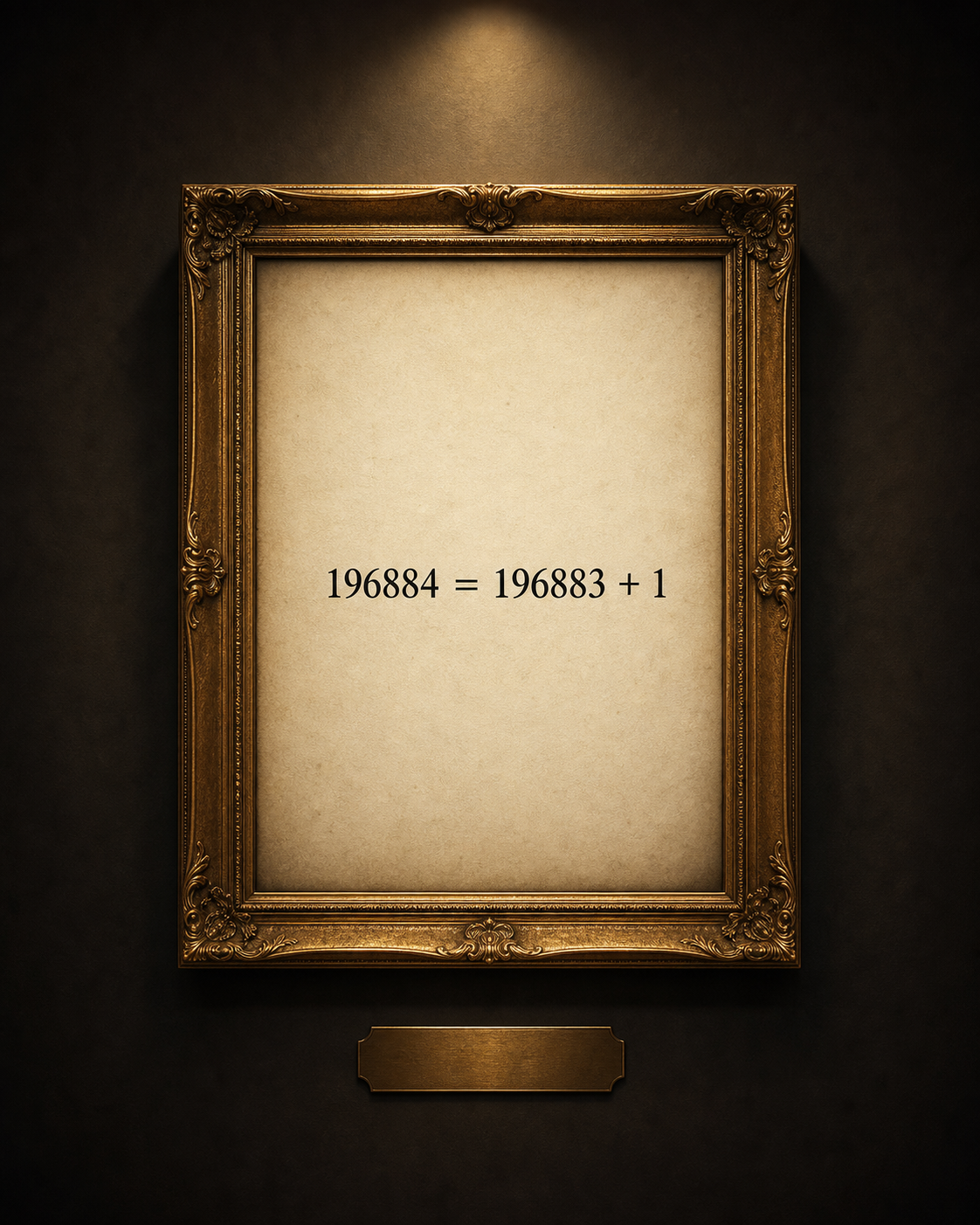
Figure · McKay’s “portrait”: photographs of McKay from his lifetime exist, but we could not find one that can be freely used. What he left the world is the coincidence itself that he recognized at a glance — . (Made by this channel.)
§2 · That old formula: what the j-function is
To understand this coincidence, we must first get to know the j-function. It has been in number theory for more than a hundred years, long an old acquaintance that “everyone can see” — only no one imagined it would get mixed up with a monster.
And to get to know j, we first need to change our angle.
2.1 Starting from complex numbers
In mathematics there is a concept called the upper half-plane:
First, what the complex numbers mean: is a complex number, that is, a point in the plane; is its real part, defined in the complex plane by the horizontal coordinate, is its imaginary part, defined by the vertical coordinate, and is the imaginary unit (). restricts this point to above the horizontal axis — hence the name “upper half” plane. But the horizontal axis itself (, called the real axis) is not included.
On the upper half-plane, length is not measured the Euclidean way, but is defined by the following formula:
In this formula, is a small step moved starting from ; is the absolute distance between two points in the plane; is read “the imaginary part of ”, that is, the of the upper half-plane mentioned above. is then the length recorded for this small step under this standard.
Plug in two points and look: at , taking a step gives ; at , taking the same step gives . For the same Euclidean length, the smaller is, the larger the reading; as , , so under this metric the real axis lies at infinity.
Area changes along with it:
is the area of a small rectangle measured the usual way (width , height ); is the area it is recorded as under this standard. Here we divide by and not by , for a very plain reason: area is the product of lengths in two directions, each direction has to be divided by once, and twice makes .
The reason for choosing this metric is: it stays unchanged under the following set of transformations. First look at this set of transformations:
is the point before the transformation, is where it lands after the transformation; are four real numbers, the four parameters of this transformation. is called the determinant of this transformation, and it governs three things, three different conditions:
- — this transformation can go back the way it came (if it equals , it cannot go back);
- — after the transformation it still lands in the upper half-plane;
- — this is a normalization: for any positive determinant, dividing all four numbers by turns it into , and this scaling does not change itself (scaling top and bottom at the same time cancels out). So requiring it to equal is not adding one more restriction; it is choosing one standard way of writing from the infinitely many ways of writing the same transformation.
One example makes all three clear together. Take ; then :
The determinant is nonzero, so it is invertible (the inverse transformation is ); the determinant is positive, so has the same sign as , and a point in the upper half-plane is still in the upper half-plane after the transformation. But in the numerator there is an extra , which is exactly . Divide all four numbers by , and the determinant becomes , while the expression for , after multiplying top and bottom by , is identical to the original letter for letter — the map has not changed, only the way of writing it, and the extra disappears.
After choosing this standard way of writing, only one doubling in the way of writing remains: and give the same transformation — in the discussed in 2.2, that takes care of exactly this. The modular group discussed in 2.2 later is the group obtained by further restricting to integers.
For such transformations, we can also derive the identities directly:
The first formula says: the height after the transformation equals the original height divided by . The second says: the small step after the transformation equals the original small step divided by . (Both formulas use the chosen above — in the general case each of their right-hand sides also carries a factor , which disappears only after the standard way of writing is taken.) What appears in both formulas is the same — this is not a coincidence; it is exactly what makes the next step work. Take absolute values and divide, and cancels exactly top and bottom:
This is an important conclusion: the left side of the equals sign is the length recorded after the transformation, the right side is the length recorded before the transformation, and the two are, remarkably, exactly the same. That is to say, every transformation in the modular group is length-preserving under this standard.
So, take a region in the upper half-plane, and with these transformations we can get many results of the same lengths; in 2.3 next we will explain further how it comes about, and here we first call them tiles:
Those tiles are each the same size. “The closer to the edge, the smaller” is only an illusion of the Euclidean coordinate system — just as on a map Greenland looks bigger than Africa.
Let us combine this with a concrete example, and take this piece:
is the real part of (that is, the above), and says “no more than half a cell to the left or right”; is the distance from to the origin, and says “outside the unit circle”. This region is called the fundamental domain. Add up the above over it (the lower limit of integration comes from , i.e. , which solves to ):
Four equals signs, each with its reason:
- Split into an iterated integral. , so the outer integral is over and the inner over .
- Integrate first. ; substitute .
- Recognize the antiderivative. .
- Plug in the limits. (because ), .
The area of every tile is , however small it is drawn. Infinitely many pieces, each with the same area.
2.2 What those two transformations actually do in the plane
If the four parameters of the set of transformations above are restricted to integers (still requiring ), what we get is the modular group, written . Read this notation piece by piece: means these four numbers are arranged as ; is the standard notation for all the integers; means the determinant is ; the in front means and are regarded as the same transformation — because after plugging into , changing the sign of top and bottom at the same time cancels out, and the landing point is exactly the same.
This whole group of transformations is generated by two transformations. Let us look at them one at a time, at where they send a point.
The translation . The whole picture shifts one cell horizontally to the right. The imaginary part does not move; the height does not change. (Corresponding to .)
The flip . (Corresponding to .) It is clearest written in polar coordinates — is the distance from this point to the origin, is its angle with the positive real axis:
The distance becomes — this is inversion in the unit circle, swapping inside and outside the circle; the angle becomes ( is the radian way of writing ) — this is reflection in the imaginary axis, swapping left and right.
So: the unit circle as a whole does not move (when , is still ), and points on the circle are only swapped left and right; the point does not move (its , , and is still ), it is the pivot of this transformation; the inside and the outside of the circle are swapped entirely.
Looking on the imaginary axis:
A point at height is sent to height . A point at height lands at height ; and (that is, ) is the fixed point. In general
— the height after the transformation equals the original height divided by “the square of the distance to the origin”. So points near the spot directly above the origin (for example points on the imaginary axis close to : is very small, and the square of is even smaller) get flung, after the division, to very high places.
and , these two, are enough to generate the whole modular group. This is a conclusion; Appendix A uses exactly it, and the main text only gives a general reading.
2.3 What a tile is: one fundamental domain, and all its transformed images
We cite the example from 2.1:
These two conditions correspond exactly to the two generators: — go any further left or right and translates you back ( translates one whole cell at a time, so half a cell is the dividing line); — go any further in and flips you out ( does exactly inversion: , a point at distance from the origin is sent to — so points inside the unit circle run to outside the circle, and points on the circle stay on the circle (swapped left and right, only does not move)).
So is “one representative of each point’s equivalence class under the modular group”. Any in the upper half-plane can be sent into by some element of the modular group, and in essentially only one way (with a few gluings on the boundary). The full proof is in Appendix A.
What is called a “tile” is all the copies obtained by applying this set of transformations to everywhere: , , , …… infinitely many pieces, pairwise congruent under the standard of 2.1, filling the whole upper half-plane.
The relation between tiles and coordinates: a point in the plane is an ordinary complex number ; a tile is not a pattern drawn on the plane, but a grouping of “which points should be regarded as the same point”. , , are, in the eyes of the modular group, the same point, so only one piece needs to be kept as the representative.
2.4 The j-function: the characteristic of an elliptic curve
The j-function is a function defined on the upper half-plane: feed it a point , and it gives back a complex number . What is special about it on this infinite tiled picture is two things.
The first: on every tile it takes the whole complex plane completely once — every complex number is taken, and each is taken only once — and it stays unchanged under all the transformations of the modular group (called modular invariant). Its meaning is defined by two:
The first equation in the first definition: move the point one cell to the right (), and the value of does not change; the second says: flip the point over by , and the value of also does not change. And 2.2 said that and generate the whole modular group — both generating transformations leave it unchanged, so the whole modular group leaves it unchanged.
The second definition is: in this position, such a function is it alone (the technical term is hauptmodul, “principal modular function”). The meaning is: any modular function (modular invariant, meromorphic, and also meromorphic at the cusp) can be written as a rational function of j — a rational function being one polynomial divided by another, of the form ; the field of modular functions is ( is the standard notation for all the complex numbers, means “all the rational functions generated by ”). That is to say, in this world, j alone is one coordinate: all other modular invariants can be computed from j. Both of these definitions (uniqueness, and how j maps the whole picture one-to-one onto the whole complex plane) are fully proved in Appendix A — including the statement, which uses only Appendix A’s own valence formula.
What was said above is what j satisfies. But what it actually is has a more accurate answer, and this answer will follow us into §3 and §4.
First take a complex number (with positive imaginary part); it gives
The meaning is: is all the integers, so means all points of the form ( ranging over all integers) — take and as two directions and walk out in integer steps, and you get an infinitely extending grid in the plane. is the set of all the intersection points of this grid, and means they are all complex numbers.
Roll up the complex plane according to this lattice (regard all points in the grid that differ by integer steps as the same point), and you get a torus — that is, an elliptic curve .
The key step: two ‘s produce the same elliptic curve (in the sense of isomorphism) if and only if they are related by the modular group:
, are two starting points; is read “isomorphic”, meaning these two curves are essentially the same one, only written differently; is “if and only if”, meaning the two sides are necessary and sufficient conditions for each other.
So that tiled picture is no longer a decorative painting. Each elliptic curve has exactly one representative point in , no more and no less. The other tiles are copies of , holding another way of writing the same batch of curves; the various ways of writing the same curve fall at the corresponding positions of the various tiles.
And the j-function is what finds a unique characteristic for each elliptic curve:
It is modular invariant precisely because all the ways of writing the same curve must be unique; when we take the whole complex plane, and take it only once, then each elliptic curve has exactly one and only one counterpart.
These two statements do not conflict; they are two sides of the same thing: the proved in Appendix A is exactly the algebraic way of writing “j is a complete invariant”. And the statement of uniqueness explains two things: why §3 suddenly starts talking about “supersingular elliptic curves”, because those are the same batch of objects over a different number field; and why in §4 the coefficients of j turn out to be “dimensions”, because the generating function of §4 is computed on a torus, and a torus is an elliptic curve — it can only depend on the curve itself.
2.5 Escher’s disk
If you feel that this picture, which gets smaller and smaller as it tiles and never repeats, looks a lot like the tessellations in the disks of M. C. Escher, that is not an illusion, and there is an exact one-line explanation of it. That transformation is called the Cayley transform:
is a point in the upper half-plane, is where it lands in the disk. Plug in two numbers and you see what it is doing: when , the numerator is , so — the “center” of the upper half-plane becomes the center of the disk; when is taken as a point on the real axis, and are a pair of conjugate complex numbers of equal length, and the result of dividing them has modulus , so the whole real axis is sent to the boundary circle of the disk. The tiles in the upper half-plane that “get smaller and smaller against the real axis” are, in the disk, the ring that “gets smaller and smaller against the boundary” — the same batch of tiles, the same standard, only drawn a different way. What Escher drew and what number theory uses really are the same thing.
2.6 That 744, and the 0 after subtracting it
We talked about the j-function earlier; when we expand j at infinity, we get the string of coefficients of §1. The variable used for the expansion is
This is derived from , one of the two generators. gives , that is, has period ; and every function with period can be written as a function of — so is not picked out; it is the unique natural coordinate. ( does not take part in this step.)
At the same time it “rolls” the upper half-plane toward infinity: writing , , so the larger ‘s imaginary part , the closer is to ; and when moves one cell to the right, the value of does not change at all (because ). The expansion starts from , and the coefficients are all integers (the first few terms are computed term by term in Appendix A.3; that all of them are integers follows immediately from Appendix A’s assembly — the leading coefficient of is ).
The standard j-function carries a constant term 744:
And what we use from here on is the version after subtracting 744:
Since the term and the term are exactly the same, the constant term changes from to . In §4 we will see that the coefficients of are exactly the “layer-by-layer dimensions” of something.
Where 744 comes from can in fact also be made clear: j can be assembled from two parts —
First make clear what “weight” is — it is about to appear in the next sentence. Weight says “how much it differs by after the transformation”. A modular form of weight satisfies
Note that it is not invariant: after the change it differs by a factor , and is the exponent of this factor. Only weight is truly invariant — the factor becomes .
Plug in numbers and look: the weight of is , so the weight of is ; the weight of is also . Divide two things of weight , and that factor is on both top and bottom and cancels:
⟹ That is written in the form “one thing divided by another” is not a contrivance: to build a function of weight , the numerator and denominator must have the same weight, otherwise that factor cannot cancel.
⚠️ But what this requirement fixes is the shape, not this one function. also has weight and is also holomorphic on the upper half-plane (differentiable everywhere in that region, with neither poles nor breaks), so also has weight — it equals (the relation between the two is the identity ). The accurate statement comes in three parts: (1) wanting weight ⟹ the numerator and denominator must have the same weight, and there is no other choice at this step; (2) further requiring holomorphy on the upper half-plane and only a pole of order one at the cusp ⟹ it can only be “weight divided by ”; (3) but what satisfies the first two is a whole family — requiring the leading term of the -expansion to be fixes ; the constant can still be chosen freely: the constant term of is what the way of writing it as computes, , while the used later takes the constant term to be .
Both are standard modular forms. is the Eisenstein series of weight 4, whose -expansion is ( is the sum of the cubes of all the positive divisors of ); is the discriminant, , with leading coefficient . The complete definitions of both, and the properties used here, are in Appendix A. Divide the -expansions of the two, and what falls out in the constant place is 744. It is computed directly from this ratio; Appendix A computes this ratio in full from the Eisenstein series. And for j’s identity as “unique”, adding or subtracting a number in the constant term does no harm. What really needs attention is, on the contrary, the 0 after the subtraction: in §4 we will see that it equals the dimension of layer 1 of the moonshine module — that layer is empty; and “layer 1 is empty” is precisely the characteristic, in §4, of “the symmetry group can only be finite, not continuous”.
§3 · “Moonshine”: one word, and a whole set of conjectures
At the end of that year, Thompson returned from Princeton to Cambridge and told this strange affair to John Conway (1937–2020) — the same Conway as in EP6. Conway had in hand a huge amount of data on the Monster, and he immediately plunged into the library, and sure enough, in nineteenth-century number-theory literature, he found the same sequence. Together with a young mathematician, Simon Norton (1952–2019), he checked it again and again: between the Monster and number theory there really was a connection, but no one could say why.
The one who gave a name to this affair that could not be explained was Conway. He called it Moonshine. The word is a double pun, and it is worth citing Conway’s own words as they are (as recorded in Ronan’s book; given here in translation):
The things we had, with no logical argument holding them up, felt like dim moonlight shining on a group of dancing Irish leprechauns. And Moonshine can also mean illicitly distilled liquor — doing this research really did have something of the flavor of illicit distilling that cannot stand the light of day.
(“moonshine” in English already has the meaning of “foolish dreaming, absurd nonsense” — this layer is the common sense; the “bootleg liquor” layer of the pun is Conway’s own joke.)
Conway and Norton wrote this set of conjectures down in 1979, under the title “Monstrous Moonshine” (Bull. London Math. Soc. 11, 308–339). What the conjecture says goes far beyond the one function j: every conjugacy class of the Monster corresponds to a modular function of its own, and each one is the principal modular function of some genus 0 group.
What the conjecture says: four words, plugging in numbers one by one
There are four words in this sentence that need taking apart. Below, each is given a definition, and then numbers are plugged in.
Conjugacy classes: why by “class” and not by “element”
and being in the same class means that there exists some in the group such that . Count it out with (all the permutations of three letters, ): the six elements fall into 3 classes:
The reason for going by class is that the trace, which the next step takes, is unchanged under conjugation — let be any representation;
Elements of the same class give the same trace, so the whole series depends only on the class, not on which element of the class was picked. The Monster has 194 conjugacy classes (the number of rows of that fingerprint table of EP7 §2 is exactly this), so there are at most 194 series.
The McKay–Thompson series : the definition, then plug in
The conjecture here first takes something on credit. Suppose there exists such a stack of vector spaces laid out in layers — this is what later became the moonshine module, written :
Read it symbol by symbol. is the direct sum, meaning the layers are laid side by side without being mixed up; is layer , a finite-dimensional space, and its dimension is exactly that string of coefficients of §1 (, , , ……). The at the upper right is read “natural”; it is the traditional notation for this object and does not denote any operation. is the Monster, and the Monster acts on each layer — every element in the group gives an invertible linear map on layer . What matters is the timeline: in 1979, when the conjecture was written down, this stack of spaces had not yet been built — its very existence was part of the conjecture; §4 will tell how it was later built.
So for each define
In the formula, the vertical bar in is read “restricted to”: regard only as that linear map on layer , then take its trace (the sum of the entries on the main diagonal of the matrix). The exponent is written rather than to shift the whole series by one place so that it starts from — aligned with the of §2.6; otherwise the two sides would differ by a factor of .
First plug in . The identity element is the identity matrix in any representation, and its trace is the dimension, , so
This step connects §1 back in. Those three identities of §1 are exactly the first few coefficients of this series split up according to the dimensions of the irreducible representations of the Monster:
The left side is , the right side is layer split into irreducible blocks. When the trace can see only the dimension; change to another , and the trace is no longer the dimension, and what we get is another series — 194 classes, so there are 194 of them.
Change the element: the same layer, another number
The step just now used only the identity element. The conjecture is about other elements, so now let us change it.
Take an element of order two in the Monster, called 2A by its ATLAS class name. The layer is still the same layer — , the dimension is still 196884, and the splitting is still the same splitting:
The only thing that changes is the element plugged in. The traces of on the two blocks are the respective dimensions of the two blocks; the traces of on the two blocks are two other numbers:
( is the character value of the -dimensional block of the representation at , read off the character table of the Monster.)
So we have the first few terms of the second series; place it side by side with the first:
How these two lines look side by side is how the whole set of conjectures looks: the same stack of spaces, the same splitting, change the element, and the whole series changes to another set of coefficients. That string of numbers in §1 that matched the j-function turns out to be only the first row of this table.
Genus 0 and the principal modular function
A group acts on the upper half-plane, and after taking the quotient we get a surface; then add the cusps back — the upper half-plane itself does not contain the cusps, and only after they are added is the surface compact — written . Genus 0 means that this compact surface is a sphere; the field of modular functions on the sphere is generated by a single function, and this generator is called the principal modular function (hauptmodul).
The first example has already been given in §2. Take ; is the surface generated from the fundamental domain as in §2.3, with that one cusp added back, and takes each complex number exactly once on (§2.4); counting the cusp in together with , “exactly once” is
that is, has genus and is its principal modular function (full proof in Appendix A; the boundary note for the general case is also there).
The second example is the one just now. The group that goes with is with a Fricke involution added, written ; in Conway–Norton’s original table it is written “2+”. Its compactified quotient is likewise a surface of genus , and is likewise its principal modular function — the function field is generated by this one function.
The group changed; the matter of “genus 0 plus one principal modular function” did not change. This shape is exactly what the conjecture says.
These functions were not made for moonshine. can be written down without mentioning the Monster at all, using only the function of number theory (OEIS files this sequence under Fricke’s 1922 textbook on elliptic functions, and links it to Ramanujan’s paper on approximating ; we did not get to these two original books, and the entries are in the sources). Moonshine did not create this batch of functions; it recognized the Monster on a batch of functions that had long lived in number theory.
A complete analysis of the conjecture
Now we can say it in full: every conjugacy class of the Monster gives a , and every is the principal modular function of some genus 0 group.
The one for we already saw in §2 — , and the group is itself; the one for we just saw — the group is . Each of the remaining ones has its own group.
A small note on counting: the 194 classes do not give 194 different series, but 171. The smallest example can be seen already on — is a commutative group, each element is a class by itself; take its representation as rotations of the plane ( rotating by ), and while : two different classes give the same trace. The mechanism is , and ; when the trace is real the two coincide. It is the same in the Monster, and it happens on every layer at once: and always share the same series, and this step brings 194 down to 172. For the last step, from 172 to 171, this article did not find the mechanism — Conway and Norton name it separately: the only other equality apart from inverses is between two conjugacy classes of order 27, and that there are no other equalities (Conway–Norton 1979, p. 310). Even in this comparison table there hides a coincidence without an explanation. (A class-by-class count is in Appendix F.)
In other words — every conjugacy class of the Monster has a principal modular function of its own.
Ogg’s other half of the riddle
In fact, nearly four years before McKay, another person had come upon the other half of the same fog.
On 14 January 1975, Jacques Tits gave his inaugural lecture at the Collège de France, and spoke of Fischer’s huge symmetry group that had not yet been built — “the Monster”. In the audience sat the Berkeley number theorist Andrew Ogg (1934– ). Ogg at the time had in hand a list of primes he had computed himself. After hearing that lecture, he compared the two sides and found them, astonishingly, exactly the same.
How that list was computed
What Ogg asked was a purely number-theoretic question: take the modular curve , then take the quotient by the Atkin–Lehner involution (when is prime, this is the Fricke involution), getting ; when does this curve have genus 0 (that is, the simplest shape, a sphere)?
The answer is a finite list. And the way Ogg himself wrote it down shows that it has structure better than listing does:
, or .
There are 11 primes with , and adding the 4 after them, 15 in all:
This whole derivation, from beginning to end, uses only number theory — modular curves, genus, involutions. It can be computed before the Monster was constructed, and in fact that is just how it was: in 1975 the Monster was still only a conjectured object; it would be truly built by Griess only in 1980 (the paper published in 1982). What Ogg himself wrote in that note was “if it exists”.
Plugging in :
First the few objects that appear here. is a modular curve, built exactly the same way as the above — take the quotient of the upper half-plane by a group to get a surface — only the group is changed to (requiring that the lower-left entry of the matrix be divisible by ). The genus is how many holes the surface has: a sphere has genus , a life ring has genus . The cusps are the few points that land at infinity after taking the quotient.
The genus of has a closed formula ( prime, two cusps):
where is the Legendre symbol: when is a square modulo it takes , and when it is not, ; count the elliptic points of orders 2 and 3 on the surface (special points fixed by some element of the group). Plug in a number and look: , because is not a square modulo (this is so for every prime ), so ; likewise , . Plug in :
Then take the quotient by the Fricke involution — it is a symmetry of order two of onto itself (do it twice and you return to where you were); take the quotient by it too, and the resulting surface is written . This step is a double cover, and the Riemann–Hurwitz formula gives the genus of the new surface ( is the number of fixed points of ; is the class number of the discriminant , that is, the number of equivalence classes of primitive binary quadratic forms of that discriminant, for example ):
These two class numbers can be obtained by directly counting reduced binary quadratic forms: , , so ,
It lands exactly on 0. And the next prime no longer does: plugging in the same way, , . So the list ends at 71, and it is not “these are all that have been found so far”: Ogg proved that after 71 the genus is never zero (this article recomputed up to 200, see Appendix C) — this is also why “the largest one is 71” is not an open case.
And on the other side, factor the order of the Monster group into primes:
The primes that appear are exactly 15, and written down they are
Identical to the list above, to the letter.
Each side can be computed independently, neither uses the other, and then they are identical to the letter. That is what makes it worth being astonished at. And Ogg in 1975 was taking a list computed perfectly clearly and comparing it with the order of a group that did not yet exist at the time.
What exactly is “super” about “supersingular”
The primes on this list are called supersingular primes in number theory.
Go back to those elliptic curves of §2.4. They live over the complex numbers; consider the same batch of equations instead over a finite field of characteristic , and most properties of the curves stay as before, but a very few behave anomalously:
- Ordinary: the -torsion points on the curve number in all (including the identity).
- Supersingular: there is not a single torsion point of order .
The endomorphism ring of a supersingular curve is especially large. In the usual case it is an order in an imaginary quadratic field; in the supersingular case it is an order in a quaternion algebra — non-commutative. “So much symmetry that it does not look like what a curve ought to have” — this is where the name comes from.
Given , there are only finitely many supersingular -invariants (about of them), and all of them fall in . The 15 primes on the list are exactly those for which these values all fall in the smaller (Appendix C).
That other half of the riddle
Look once more at the end of the list: 47, 59, 71. The last episode said that these are exactly the three largest prime factors of the order of the Monster, and their product is exactly 196883 — the number McKay recognized had been lying all along at the tail of Ogg’s list.
Ogg simply wrote this coincidence into the paper he was writing at the time (in a Remarque, not a theorem), offering a bottle of whiskey as a reward for an explanation. (What he wrote in the original was Jack Daniels, without the apostrophe; the distillery’s official spelling is Jack Daniel’s. When quoting his original words we follow the former.) When McKay made his observation nearly four years later, the reward of this bottle was still open — and to this day (2026), no one has cleanly claimed the bottle.
He told this strange affair to Tits and to Serre (Jean-Pierre Serre, the one who wrote A Course in Arithmetic), and Serre’s reaction was a single “Sans blague” (no kidding). No one had the slightest idea why it should be so.
This riddle and the riddle of moonshine itself are two different matters, and must be looked at separately. First, which half is settled: the list of supersingular primes itself — including “the largest one is 71”. It is a classification result that Ogg computed from the side of modular curves: once exceeds 71, the genus of is no longer zero, and the list stops there. What hangs open is why the two lists are equal. Moonshine proved one direction of it — “a prime divides ⟹ it is a supersingular prime” (so a prime greater than 71 certainly does not divide ); but the other way round — why each one of the 15 primes on the list happens to divide , and why the prime factors of the Monster happen to reach exactly up to 71 — to this day there is no conceptual explanation; this is an independent unsolved riddle. (See Appendix C for details.)
§4 · The proof: the moonshine module, and a string theory
The conjecture was sitting there, matching term by term, but why did it match? No one could say. And the road that can at present be called an explanation is understanding it with the help of physics.
The moonshine module V♮
First comes the first step, completed by three mathematicians, Frenkel, Lepowsky and Meurman (FLM). They built a space — first announced in 1984, written up in 1988 as the book Vertex Operator Algebras and the Monster — and this space brings two properties together: its layer-by-layer dimensions are exactly the coefficients of ; and its symmetry group is exactly the Monster. This space is called the moonshine module , and its structure is called a vertex operator algebra (VOA). The stack of spaces taken on credit in §3 was only here truly built.
In , that is the natural sign of musical notation, read “natural” — it takes part in no operation; it is only a proper-name marker. as a whole is read “the moonshine module”, and refers to exactly the one particular space below.
In physics there is a concept called conformal field theory. A field theory describes “what is vibrating at each point of space”; conformal is a requirement added on top of it: enlarge, shrink or bend the whole picture arbitrarily, and as long as the angles everywhere are unchanged, this theory cannot tell the difference between before and after. ⟹ It has no built-in unit of length; “how big” carries no information for it. Two dimensions is the setting where this requirement is most powerful: the local angle-preserving transformations in two dimensions are so many that they form an infinite-dimensional symmetry, strong enough to almost pin down the theory itself; whereas in dimensions, such transformations form only a finite-dimensional group — two dimensions is the only exception. The theory in this episode has two identities: mathematically, its axiomatization is the VOA to be described below; physically, it lives on the surface swept out by a string (see the “worldsheet” later in this section).
A vertex operator algebra (VOA), then, is the structure that writes “two-dimensional conformal field theory” as axioms. Concretely, it is a graded vector space
( is the direct sum, laying the layers side by side without mixing them up), plus one rule: each state is paired with an operator
is called the vertex operator of ; is not a number but a formal variable, used only to number a string of operators ( is read “‘s -th mode”; it sends one state to another state). In this structure there is a special element , which gives an operator and a number : is responsible for the grading (layer is those states for which the eigenvalue of is ), and is called the central charge. ⟹ A VOA is the rigorous version of the “operator product expansion” of string theory (the physics-side account is in Appendix E, the mathematics-side axioms in Appendix D.1; this section uses only the two points “grading + each layer is a representation of the Monster”).
The “+1” of §1 here acquires an identity: the layer-by-layer dimensions of are the coefficients of , and the Monster acts on it — the two things are no longer a numerical coincidence across empty space, but two faces of the same object.
“Layer by layer” deserves a sentence of expansion. The dimension of layer is exactly the coefficient that sits, in , in the place — layer 1 corresponds to the in the constant place, layer 2 to the place’s , and so on (that leading ‘s coefficient also has an identity: layer 0, the vacuum, one-dimensional). And the Monster acts on each layer separately — so each layer is itself a representation of the Monster. Look at layer 2: it is 196884-dimensional, and split up it is exactly the one-dimensional trivial representation the 196883-dimensional smallest representation — McKay’s “+1” is the one-dimensional trivial direction in this layer. The additions that Thompson did back then when he “tried the next coefficient” acquire a geometric meaning here: that was splitting the representations layer by layer (the three identities of §1 are exactly the splittings of layers 2, 3 and 4).
The key is where the words “vertex operator” come from — they come from physics, from string theory. In the preface to their 1988 book, FLM say it very plainly (translated from the original English preface; given here in translation):
Our main theorem can be read as a quantum-field-theoretic construction of the Monster; in fact, what it says is: the Monster is the symmetry group of a certain special string theory.
This is the part of this episode written for readers in theoretical physics (the conceptual development is in Appendix E; here only the picture is given).
Where that 24 comes from. The critical dimension of the bosonic string is ; after light-cone gauge fixes away one pair of coordinates, transverse oscillators remain — where comes from (several different roads point to the same ) is in Appendix E.1, and the main text does not repeat it. It is precisely these 24 directions that need to be compactified, so a 24-dimensional lattice is needed.
Take the Leech lattice (the lattice of EP6). What is special about it is that it has no “roots”, roots meaning lattice vectors of squared length 2:
Two words are needed here. Even says that the squared length of every vector in the lattice is an even number; unimodular says that the determinant of the lattice is — an equivalent statement is that this lattice and its dual lattice are the same one. These two conditions pin things down extremely tightly: there are only 24 even unimodular lattices in 24 dimensions in all (this list is called the Niemeier classification, settled in 1973), and the other 23 all have roots; Leech is the only one that does not.
How is it constructed? Compactify these 24 bosons on the torus built from , and you get a vertex operator algebra ; then fold away one symmetry:
In the formula above: is the symmetry obtained by negating lattice vectors () and lifting it up; the superscript is read “take the part invariant under ”, that is, those states that stay exactly as they are after being acted on by ; the superscript is read twisted, and is the unique “twisted sector” of this symmetry. ⚠️ This is not as simple as “divide by ”: one must both project onto the invariant part and attach the twisted sector — taking only does not give (Appendix D.2).
The coincidence 196884 is assembled
What is most worth noticing about this construction is here: is not a parameter tuned to match ; it is the result of adding two parts. Count layer 2 —
The untwisted half: the -invariant states are of two kinds: lattice vectors of squared length 4 ( and paired up, each pair giving one invariant combination), and the symmetric square of the 24 directions:
⚠️ The “weight” here and the “weight 4” of §2 are two different quantities. The weight of §2 is the exponent that appears extra after a transformation; the weight here is the layer number — that number of layer 1, layer 2; it says only which layer this state sits in. That both places happen to be called “weight” is a collision of historical naming; when reading, understand each according to its own sentence.
The twisted half: the ground state of the twisted sector is -dimensional, at weight ; add one more mode to rise to weight , and there are 24 directions that can be added:
Adding the two halves:
Every number on the left comes from the lattice and the construction itself; the right side is ‘s coefficient in the place. This step uses no information whatsoever about the -function from start to finish.
Why layer 1 must be empty
Layer 1 of a lattice VOA has only two sources — roots, and the dimension of the lattice:
And acts on these 24 directions exactly as , so not a single one is invariant; and the twisted sector starts only from weight and cannot reach weight . So
This step is the core, and the whole chain of logic is:
( is read “automorphism group”, meaning all the symmetries that keep this structure unchanged.) Why the middle step holds: the states of weight 1 are exactly the generators of continuous symmetries — each one gives a direction of a Lie algebra, along which one can rotate continuously. When layer 1 is empty, there is not a single continuous direction, the dimension of the symmetry group is , and so it can only be a finite group (strictly speaking one also needs: such automorphism groups are algebraic groups, and an algebraic group of dimension must be finite) — and this finite group is exactly the Monster.
Change the lattice and the conclusion no longer holds, and this can be verified. Take any of the other 23, for example — three copies of placed side by side. In , the vectors of squared length equal to number (such vectors are called “roots”), so three copies have ; whereas Leech has :
As said earlier, there are 24 even unimodular lattices in 24 dimensions in all, and only Leech among them has roots. Back to : after folding, layer 1 is , and the continuous symmetry comes back. And layer 2 is still — has fewer vectors of squared length than Leech ( versus ), fewer, which after halving is states, made up exactly by the states of “one root plus one oscillator”. Change the lattice, and not one of the other coefficients of changes; the only thing that changes is the constant place. (This is not a coincidence: modular invariance pins down all the coefficients other than the constant place; see Appendix E.3.) So what singles out Leech is not , it is that .
The “vertex operators” of this conformal field theory are exactly the operators of string interactions. And the most crucial point is: the partition function of this conformal field theory on a torus (that is, the generating function of its layer-by-layer dimensions) is exactly (the rigorous statement requires Zhu’s theorem; see Appendix E). So “why the j-function should happen to be a modular function” gets a clear explanation on the physics side — the modular invariance of the worldsheet torus; this phrase needs to be taken apart. A point particle moving in spacetime draws a line, called a worldline; but a string is not a point, it is something with length, and what it sweeps out as it moves is no longer a line, but a two-dimensional surface — this is called the worldsheet. All the calculations in string theory finally come down to “what happens on this surface”.
Next look at the shape of the surface. A closed string is a loop, and what it sweeps out when it propagates freely is a cylinder; and when this process is joined end to end — the string goes around one whole trip and returns to the state it started from — the two ends of the cylinder are glued together, and only then is what we get a torus (the surface of a doughnut). What needs computing is exactly this.
And the word “torus” has already appeared in §2.4: there it was the torus obtained by rolling up the complex plane according to the lattice , its shape described by one complex number (in the appendices the same quantity is written ; it is the same thing). That sentence of §2.4 now comes into use a second time: two ‘s make the same torus if and only if they are related by the modular group. In other words, the same worldsheet can be labeled with different ‘s, and what separates these different labelings is exactly the action of . Since physics recognizes only the surface itself, and not which you chose to label it with, the quantities computed on this surface must be invariant under — that is to say, it must be a modular function. The symmetry of §2.4, which looked like a convention internal to number theory, here becomes a rule that physics must obey. That old formula of number theory, more than a hundred years old, is in fact related to a special kind of string theory.
⚠️ But we cannot stop the statement here: modular invariance is a threshold, not a sieve. It requires the answer to be a modular function, but does not tell you which one — there is more than one candidate that clears this threshold. What really picks out from among them is the independent fact of construction above: layer 1 is empty. The rigorous statement is in Appendix E.3.
Borcherds’s proof, and the Fields Medal
The one who pushed FLM’s construction on to “proving the whole conjecture” was Richard Borcherds (1959– ) — when the moonshine module was announced, he was still a doctoral student under Conway. He built a new class of infinite-dimensional Lie algebras (today called Borcherds algebras), and picked out from them one key special case — the “Monster Lie algebra”, making use of the no-ghost theorem of string theory (Goddard–Thorn, 1972). In 1992, in the paper “Monstrous moonshine and monstrous Lie superalgebras” (Invent. Math. 109, 405–444), he completely proved the Conway–Norton conjecture: every McKay–Thompson series is indeed the principal modular function of a genus 0 group.
The difficulty of the conjecture is: on one side is a group, on the other side are functions. On the Monster side there are 194 conjugacy classes, on the number-theory side there are 171 series, and the Conway–Norton conjecture assigned a series to each class — but there was no reason at all for “why they match”; you had nothing in hand that could carry the information from this side to the other side.
What Borcherds built was exactly that bridge. His approach was not to check those 171 series coefficient by coefficient (each one has infinitely many coefficients; that could never be finished), but:
First build a “Lie algebra” from . A Lie algebra is something that appeared in EP4 — the set of “infinitesimal generators + commutation relations” that describes continuous symmetry. The one he built (he called it “the Monster Lie algebra”) has two properties, and neither can be missing:
- It remembers the Monster: the Monster acts on it, so its numbers everywhere carry the Monster’s information;
- It remembers : this class of Lie algebras (generalized Kac–Moody algebras) each come with a “denominator identity” — its structure list can be written down completely in two ways: one written as a product, one written as a sum; the two ways of writing describe the same thing. And the denominator identity of this one is exactly that product formula for already written down long ago in number theory.
The link is this one identity. The same algebra, seen from the group side, is a representation of the Monster; seen from the number-theory side, it is the expansion of . What remains is to “twist” this identity once — twisting once for each conjugacy class — and one gets all 171.
Therefore, he did not prove, one by one, what each of those 171 series equals; he built a thing that ties them together, whereby each series is pinned down by its first few coefficients, and what is left is only one finite check.
The skeleton has four steps, and each step is given a formula one can look at (Appendix D.3 has five steps, cut differently from here).
① Build a Lie algebra. Tensor with another vertex operator algebra and take its physical states:
is a German blackletter m, read “the Monster Lie algebra”; is a two-dimensional even unimodular Lorentzian lattice, the central charge of whose vertex operator algebra is , so together it is — the same 26 as the critical dimension (for why, see Appendix E). ⚠️ It is , not the Leech route; the latter gives a different algebra (Appendix D.3).
② This step is what the no-ghost theorem refers to. Goddard–Thorn identify, in , the physical states of momentum with a certain whole layer of — and the isomorphism is as representations of the Monster, not just equality of dimensions. So the “root multiplicities” of the Lie algebra can be expressed as:
( is read “multiplicity”, meaning how many linearly independent elements there are in the direction of this root; is, of , the -th coefficient.) Plug in a concrete root :
The same 196884; this is its third identity in this episode — the left side of McKay’s equation, ‘s coefficient in the place, and now the multiplicity of a root.
③ The denominator identity. The “denominator identity” of this class of Lie algebras is an identity that writes its structure as a product equal to a sum. The one for is exactly the Koike–Norton–Zagier product already known in number theory (the here is only shorthand for and has nothing to do with the denoting a prime):
The left side is two values of subtracted, the right side is an infinite product, and the exponents are exactly those multiplicities above. The structure of the algebra and the arithmetic of are, in this one line, forcibly pressed into the same thing.
④ Only by twisting do we get all 171. The one above is the untwisted version; it recovers only the one for (that is, itself). What really gives all the is the “twisted” denominator identities, one for each conjugacy class — replace the dimensions in the formula above by the traces . “Twisting” is the key, not a footnote: what it gives is exactly the replication identities proposed by Norton (1984).
Closing up: complete replicability determines each uniquely by the first 5 coefficients of it (together with the various powers of ), and what remains is one finite computer check — so for the 194 classes and 171 series, every one lands on a principal modular function of genus 0.
In 1998, Borcherds received the Fields Medal for this (and related work) (at the International Congress of Mathematicians in August, Berlin), and the citation named moonshine.
About how he felt on receiving the prize, in the year he received it he said something to Simon Singh, who interviewed him. In translation, the gist: he said he did not really feel anything special; before receiving the prize he had always thought it was enormously important, and now he understood that it did not mean anything. But — at the moment he proved the moonshine conjecture, he was so happy he flew to the moon (“I was over the moon”). The prize is cold; the proof is warm. And over the moon literally means “up on the moon” — the man who proved moonshine said of himself that he had gone up on the moon.
The vertex operator algebras, generalized Kac–Moody algebras and the no-ghost theorem of string theory used in the course of the proof are a true high peak, and a blog appendix certainly cannot cover all the details, so here we pass over it in a stroke. So this episode cites it honestly and does not rebuild it: Appendix D gives the skeleton on the mathematics side (VOA, , Borcherds’s strategy), and Appendix E gives the conceptual picture on the physics side. We prove to the end what can be proved (Appendices A, B), and state plainly what we cannot prove.
Coda · Proved, yet still a mystery; and a road walked for two thousand five hundred years
Moonshine has been proved; Borcherds’s theorem holds.
But “proved” and “understood” are indeed two different things. Why the Monster, why modular functions, why precisely the Leech lattice, why every series of that family is genus 0 — string theory has given the best clue so far (the modular invariance of the worldsheet, which connects the number-theory side and the symmetry side), but that is not a complete explanation. Ogg’s half of the riddle, the reverse direction, still has no resolution to this day (that is another riddle — why the two lists are equal; there has never been a conceptual reason); and that bottle of Jack Daniel’s has still not been claimed by anyone. This, perhaps, is what is most mysterious about it.
So this series too has come to its end. Let us look back once at this road:
From the five regular polyhedra in the hands of the ancient Greeks, asking “why are there only five”, the starting point was a geometric fact — there are exactly five regular polyhedra; the ancient Greeks counted them, but did not know that what they were counting was in fact symmetry. More than two thousand years later, Galois, to answer “why the quintic equation has no root formula”, made symmetry into an object that can be operated on — the group. Once there was an object, there was the next question: break all finite symmetries down until they cannot be broken further, and count these “atoms” clearly. Counting from Galois, it took more than a hundred years, and the answer is: eighteen infinitely extending families (exactly what EP5 took stock of), plus 26 sporadic groups that no family can take in (the box EP6 opened) — the largest of them is the Monster. The last step was one nobody expected: this largest exception matches, term by term, an old formula of number theory more than a hundred years old; this correspondence was proved to hold by Borcherds in 1992, and why it holds, no one to this day can say. From “why exactly five” to “why exactly a match” — the starting point and the end point of this road are the same kind of question.
Humankind has chased this thread of “symmetry” for two thousand five hundred years, from the regular polyhedra the ancient Greeks drew in the sand, to a monster living in over a hundred thousand dimensions, gazing across space at the depths of the whole of number theory. It did not stop at a full stop of “at last we understand it all”, but stopped before a riddle that can be proved, yet still cannot be understood.
The twenty years after the book
Ronan’s book stops at 2006. In these twenty years the riddle has not been solved — on the contrary, it has grown bigger.
In 2010, three physicists — Tohru Eguchi, Hirosi Ooguri and Yuji Tachikawa — came upon the same kind of coincidence in a completely different place: computing a function on the K3 surface (a standard geometric stage in string theory) — the elliptic genus — they found that the expansion coefficients decompose term by term into the dimensions of representations of M24 — the largest of the five Mathieu groups of EP6. This correspondence itself was rigorously proved to hold by Terry Gannon in 2012; but it is even more “mysterious” than Monster moonshine: Monster moonshine at least has the moonshine module as a “home”, while Mathieu moonshine has not even found its “home” yet — it has been proved that no concrete K3 model really carries this M24 symmetry, yet the correspondence is sitting there plain as day. The paper that discovered it writes, in the last sentence of its own abstract: “The reason is yet a mystery.”
Then they came in batches. In 2012, Miranda Cheng, John Duncan and Jeffrey Harvey found that Mathieu moonshine is not an isolated case, and named it umbral moonshine; then (2013) this family of phenomena was counted up as a family numbered one by one by the 23 Niemeier lattices; by 2015, the existence of the “moonshine modules” for all 23 cases had been proved — the Mathieu case first proved by Gannon, the other 22 cases completed together by Duncan, Michael Griffin and Ken Ono. However, these proofs give abstract existence; in most cases there is not even an explicit construction yet.
In 2017, moonshine reached the other side of that dividing line of EP6: among the 26 sporadic groups, there are 6 “pariahs” that even the Monster cannot take in — now the moonshine of one of them, the O’Nan group, has also been proved (Duncan–Mertens–Ono, 2017, the paper published in Nature Communications), and this time what was given was an explicit number-theoretic theorem (class numbers and the arithmetic of elliptic curves) — the proof landed, and the “why” is likewise still empty. Even groups not inside the Monster have been lit by moonshine.
Looking back now, “moonshine” is no longer an isolated case but a family — Monster moonshine, Mathieu moonshine and the umbral family behind it, pariah moonshine, and beyond these more small branches. Yet in this family, the “why” of not a single member has ever been truly explained. The clues on the physics side are also multiplying: in 2016 there was work that gave, starting from string theory, a physical derivation of the genus-0 property — but the authors themselves marked its mathematical level as a “sketch”. The clues are more and more, but the question itself has become more and more mysterious. So in 2026 this is still in the present tense: it can be computed, it can be proved, but no one can say why.
Perhaps this is the fitting ending. The best moments of mathematics have never been “we know everything”, but “we know that something is here, yet do not yet know why”.
The box has been opened, the monster has appeared, moonshine has been proved. And where exactly that beam of moonlight comes from — that is left to the future.
(The Symmetry and the Monster series · The End.)
Author’s note · Closing
As the end point of this series, let me say what I have felt over these few months. First, AI can help me do so many things I had not thought of before, or had thought of but had no way to realize; this video series is one of them. Second, in these short few months I have indeed experienced anxiety and bewilderment such as I have never had before; it comes from the difficulties in my life that I am currently facing, and also from the perplexities AI has brought. After finishing this series I still have many topics I want to do, such as relativity, such as quantum mechanics, and also such as a series on the Nobel Prize in Physics. I hope that you who have read this far will give me lots of support. Thank you.
Appendices A–F (mathematics / physics)
Table of notation (common to Appendices A–F)
The main text assumes by default that the reader has undergraduate mathematics, and the notation below basically does not appear in undergraduate courses. It appears again and again in A–E, so it is gathered here and explained clearly once; when it is first used in the later sections it is not explained again. When you cannot read on, come back to this table; do not guess.
The modular-forms side (A / B / C)
| Notation | Read as | In one sentence |
|---|---|---|
| · | upper half-plane | ; is it with the cusps added |
| cusp | cusp | that “point at infinity” ; only with it added is the quotient surface compact |
| weight | weight | the exponent in the transformation law ; means “completely invariant” |
| meromorphic | meromorphic | holomorphic everywhere except at isolated poles |
| cusp form | cusp form | a modular form that takes the value at the cusp ( is one) |
| “the order of at “ | zeros count positive, poles negative: a zero of order is recorded , a pole of order is recorded , and if there is neither it is | |
| divisor sum | each of the positive divisors of raised to the -th power, then added, e.g. | |
| Riemann zeta | used only to normalize into the version with leading term , | |
| stabilizer | stabilizer | those group elements that fix a certain point in place; the stabilizer of has order , that of order |
| argument principle | argument principle | counts the number of zeros minus the number of poles inside the contour |
| · · | modular curves | the compact surfaces obtained by taking the quotient of by the corresponding groups; |
| Fricke involution | a transformation of order two that folds in half (acting twice returns to where it was) | |
| class number | how many equivalence classes of reduced primitive binary quadratic forms of discriminant there are | |
| genus | genus | the number of “holes” in a surface: a sphere , a torus |
| The vertex-operator-algebra / physics side (D / E) |
| Notation | Read as | In one sentence |
|---|---|---|
| ”V natural” | is the natural sign of musical notation; it takes part in no operation and is purely a proper-name marker | |
| · central charge | L-zero · central charge | the eigenvalues of give the grading (layer ); is a number that comes with this structure |
| · | trace · “the trace of restricted to “ | regard only as a linear map on layer and take the sum of the main diagonal of the matrix |
| German blackletter m | the Monster Lie algebra | |
| · | even unimodular Lorentzian lattices | the subscripts are the signature (how many plus and minus signs); the former has , the latter |
| multiplicity | how many linearly independent elements there are in the direction of this root | |
| automorphism group | all the symmetries that keep the whole structure unchanged | |
| an oscillator acting on the vacuum | is the vacuum state; excites it to a higher layer | |
| -cofinite | C-two cofinite | a finiteness condition on a VOA, one of the premises of Zhu’s theorem |
| GKM | generalized Kac–Moody | the class of infinite-dimensional Lie algebras that Borcherds algebras belong to |
| DDF · BRST | DDF states · BRST | the former is a standard construction of the transverse physical states; the latter is an equivalent quantization criterion |
Appendix A (full proof) · The -function and the modular group acting on the hyperbolic plane
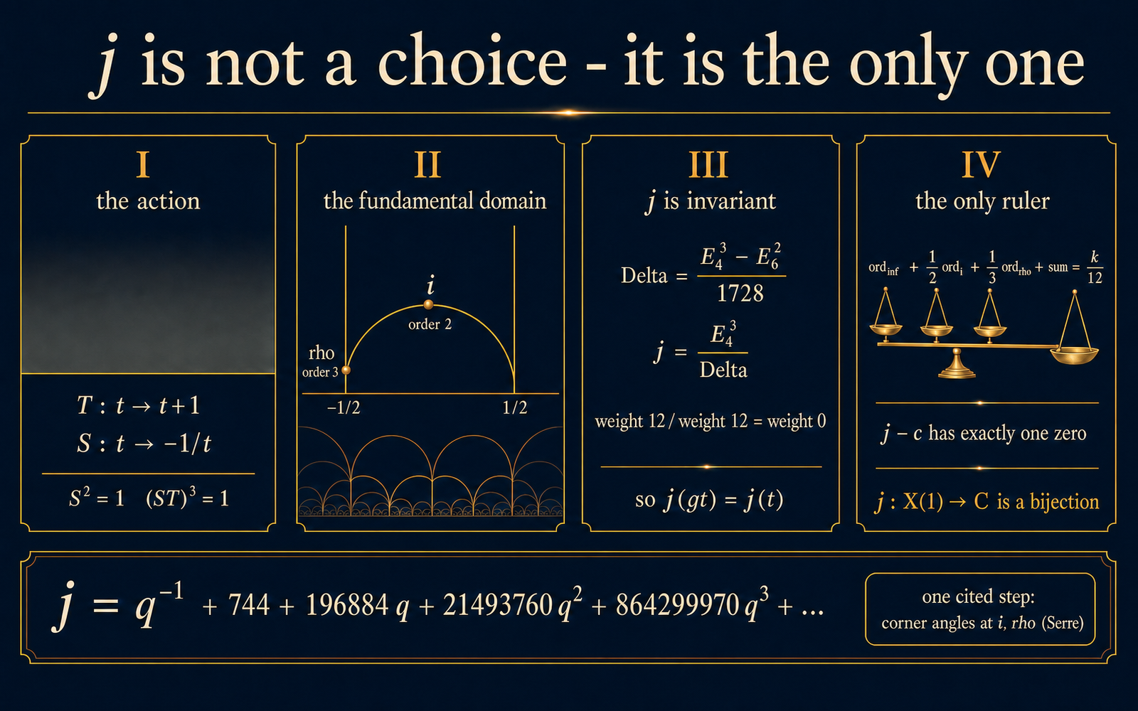
Appendix A concept diagram · The modular group cuts the upper half-plane into congruent tiles: the standard fundamental domain is held between , its bottom edge is an arc of the unit circle ( at the top of the arc, at the left corner); the j-function sweeps the whole picture completely once on each tile — the unique principal modular function (hauptmodul) in that position. (Made by this channel · mathematical infographic)
What this section is to do. The main text, §2, says “to understand the coincidence 196884, first understand ”. Here is explained to the bottom: how the modular group acts on the hyperbolic plane (the upper half-plane), what its fundamental domain looks like, why is modular invariant, and, most important, one sentence — is not “some” modular invariant function; it is the unique one in that position (hauptmodul). This sentence is proved to the end with the valence formula. Everything this section covers is classical modular form theory; except for three steps marked as cited, the proofs are all written out.
What each of the four subsections delivers (look at this row before entering any subsection, and you will not lose track of where you are in the middle of a proof):
| Delivers | What the next subsection does with it | |
|---|---|---|
| A.1 | how the modular group acts, the two generators and | A.2 uses them to send any point into |
| A.2 | the fundamental domain exists and is (in its interior) unique, plus the two elliptic points | in the valence formula of A.4, what carry, , comes from here |
| A.3 | is modular invariant, and its -expansion coefficients can be computed by hand | A.4 needs only one fact from it: has a simple pole at the cusp |
| A.4 | is a bijection ⟹ genus , is a hauptmodul | the “each complex number is taken exactly once” of §2.4 in the main text, the “principal modular function” of §3 |
A.1 The action of the modular group (full proof)
The upper half-plane . The integer modular group
acts by Möbius transformations: . The key identity (computed directly):
so is indeed preserved. act trivially, so what actually acts is . The two generators:
satisfy , (in ). ” generate ” is a by-product of the proof about the fundamental domain below.
A.2 The fundamental domain (full proof)
Proposition. is a fundamental domain for the action of : (existence) every orbit meets at least once; (uniqueness) two different points in the interior of are in different orbits.
Proof. (Existence) Take . On the orbit , ; for fixed , only finitely many pairs make smaller than any given bound ( is a point of the lattice , which is discrete), so has a maximum on the orbit; call a point attaining it . Translate by so that (this does not change ). If , then , contradicting maximality; so , that is, . (Replace the orbit by the -orbit, and the argument holds word for word, so this step also shows that can already send any point into ; combined with uniqueness this gives .)
(Uniqueness) Suppose are both in and ; without loss of generality , that is, . Since we have , and , so . Case by case: when , , and on both sides together allows only (unless is on a vertical boundary , in which case glues one vertical edge to the other); when , restricts to the arc , and glues the left and right halves of the arc to each other. Both kinds happen only on the boundary; the interior of is therefore unique point by point.
(Elliptic points: is fixed by , with stabilizer of order ; is fixed by , with stabilizer of order . The stabilizers of the other points are trivial. The “fractional weights” of these two points go straight into the valence formula.)
A small example (sending a concrete point into , in three steps). Take (its imaginary part is only , far from ). Follow the algorithm given by the existence proof above:
- (shift left by ): ; the real part enters ;
- , use : . Note that the imaginary part jumps from to — exactly the magnifying mechanism in the proof (here magnifying by a factor of );
- (shift right by ): — neither more nor less, it lands on the elliptic point .
The composite matrix , ; a one-step check: (already verified with exact fractions, including every intermediate step).
A.3 is modular invariant (full proof, via Eisenstein)
The Eisenstein series of weight ( even)
Rearranging the summation index by ( is a lattice automorphism) gives directly the weight- transformation law
Normalize ; its -expansion () has integer coefficients (cited: Serre VII):
The discriminant and (the second equals sign is the Jacobi product formula, cited: Serre VII):
is a cusp form of weight ; is nonzero everywhere on (every factor is nonzero, and when , converges, so this infinite product converges to a nonzero value), and it has a simple zero at the cusp . So : the numerator has weight , the denominator has weight , and the quotient has weight — that is, , is a modular invariant function; it is holomorphic on (), and has a simple pole at the cusp (the simple zero of , ).
A small example (multiplying out and by hand). The main text, §2, says ” is computed from the Eisenstein series” — this computation uses only the two lines of expansion above, and can be completed by hand going up to . The numerator:
(: ; : . Here .) The reciprocal of the denominator:
(Counting by : for take one copy of , ways; for take two copies of ( ways) or one copy of ( ways), in all.) Multiply the two strings and multiply the whole by :
was not picked by anyone; it is . The higher terms the same way (the intermediate coefficients and the totals were all checked by program):
A.4 is a hauptmodul (full proof, valence formula)
Take the quotient of by and add the cusp , and we get the modular curve . What is to be proved is:
Theorem. is a bijection (the cusp corresponding to ). Equivalently: has genus , and is its hauptmodul (a single generator, field of modular functions ).
The tool is the valence formula (the formula). For a modular form of weight , meromorphic on and at the cusp, ,
The in the sum ranges over the equivalence classes of points of under the action of the modular group (except the two classes of and ), each class counted only once: points on the boundary of glued together by , count as the same one, and and are also the same class. How to read it: the left end is the total amount of zeros (counted with discounts at ); the right end is determined only by the weight . In other words, how many zeros a modular form can have is decided by its weight — this is why below can only be a bijection.
First look at how this formula is used, with three examples (the row uses the conclusion of A.3; the proofs of and are in the small example below and use only the transformation law):
| weight | already known | left end | ||
|---|---|---|---|---|
| simple zero at the cusp, nonzero everywhere on (A.3) | ✓ | |||
| (small example below), that is, | at least | |||
| (small example below), that is, | at least |
The first row is a check: both sides are . The last two rows, however, use the formula to derive new information: , are holomorphic on and at the cusp, so every term on the left end is not less than ; since is at least and already uses up the , the zero of at must be a simple zero, and it has no other zeros in — this was not looked up; it is pinned down by this formula. (For contrast: if had a zero of order two at , the left end would be , and the formula would fail on the spot.)
Proof (the valence formula, compact contour version). Integrate , the contour taken as the boundary of : along the arc at the bottom, the vertical edges on the two sides, a high cut line at the top, with small notches made to go around and the cusp. The argument principle computes the left end as the sum of zeros and poles in the interior of , . The pieces of the boundary cancel in pairs: the two vertical edges are glued by and their contributions cancel; the left and right halves of the arc are glued by , makes , and the extra integrates along the arc to ; the top cut line gives the cusp term (, and corresponds to going once around ); the central angles of the three small notches: at , ; at and , each, in total, contributing respectively. Combining gives the formula. (This step is cited: the notch angle amounts at , , come from these two points being folded by the stabilizers ; the segment-by-segment accounting of angles in this step would take up half a page if expanded, so here the conclusion is stated and Serre’s A Course in Arithmetic VII §3 / Apostol Ch. 2 are cited; all the other steps of this proof are written out above.)
Proof ( is a bijection, using valence). Take and look at . It has weight , is holomorphic on , and has a simple pole at the cusp (coming from ‘s ), that is, . Substitute into valence ():
The right end is and , so the total amount of zeros in the interior of (with the weights at ) is exactly . Since is holomorphic and all , this “total of ” can only be realized by exactly one ordinary zero (weight ), or a zero of order two at (weight ), or a zero of order three at (weight ) — whichever it is, , in , takes the value exactly once. is arbitrary, so is both injective and surjective (the cusp corresponding to ).
Corollary: has genus ; every modular function is a rational function of (field of modular functions ) — is a hauptmodul. This is exactly the precise meaning of ” is the most natural one in that position”.
Proof (of the corollary, using only the valence formula proved above). Let have weight , be modular invariant, and be meromorphic on and at the cusp. has only finitely many poles in the fundamental domain (near the cusp this is controlled by “meromorphic at the cusp”, and in the remaining part the poles have no accumulation point); let take the values at these poles. Take large enough; then is holomorphic on (by the theorem above, is zero exactly at the corresponding pole, and multiplying enough times cancels it; overdoing it only adds zeros, which is harmless). has at most a pole of finite order at the cusp: since , powers of can match the principal part at the cusp order by order, so there exists a polynomial such that is also holomorphic at the cusp. If is not constant, take any : is holomorphic everywhere (including the cusp) and has a zero at — substitute into the valence formula (, the right end is ): every term on the left end is and at least one term is , a contradiction. So is constant, , and .
(Along the way, prove that sentence of §2 in the main text, “adding or subtracting in the constant term does no harm”: the translation is an automorphism of ; a bijection a bijection, — is likewise a hauptmodul.)
The boundary of the general case. The main text, §3, says that every McKay–Thompson series is the principal modular function of some genus-0 group. This statement, used for a general group , uses the classical correspondence for compact Riemann surfaces — the quotient surface has genus ⟺ the function field is generated by a single function (). The general case needs machinery at the level of Riemann–Roch, beyond the scale of this episode, and is cited, not proved (a standard textbook result on Riemann surfaces). What this section proves in full is the key instance (the theorem + corollary above), that is, the most important stop of this correspondence in moonshine.
A small example (two anchor values: , — the elliptic points of A.2 connect up here).
- : fixes , and the weight- transformation law gives , so . From we get , so . And the simple zero of , once squared, becomes a zero of order two, matched with ‘s weight — exactly, of the “total of ” in the bijection proof, the realization.
- : gives , so the weight- transformation law plus -periodicity: , and , so , — a zero of order three matched with the weight , the kind.
The two values were additionally checked numerically by program (the -series summed at and respectively, truncation error ). On one picture three things line up at these two points: the fixed points of A.2, the fractional weights of valence, and ‘s anchor values and .
What in this section is proved and what is cited: the formula for , (in ), the existence and uniqueness of the fundamental domain — the proofs are all above. The coefficients of in their -expansions were computed independently by program from the Eisenstein series, and the two ways of writing , and , agree term by term (this is a check of finitely many terms, not a proof). This article does not prove, and cites directly, three things in total: ‘s -expansion, the Jacobi product , and the step of the angle amounts at in the valence formula, all found in Chapter VII of Serre’s A Course in Arithmetic. The three small examples were also checked by program: the matrix that moves the point, , verified with exact fractions (including every intermediate step and ); the hand-multiplied intermediate coefficients and the decompositions of and ; the numerical values , (series taken to terms, error less than ).
Appendix B (full proof, continuing EP7 Appendix B) · The moonshine arithmetic identities
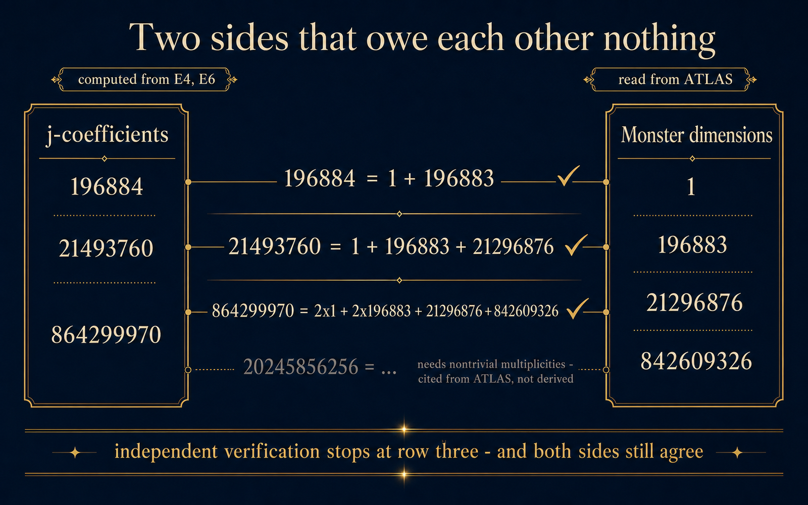
Appendix B concept diagram · The comparison table of the moonshine arithmetic identities: on one side the coefficients of the j-function (computed independently from Eisenstein), on the other side additions of dimensions of Monster representations; the first three match term by term (starting from ); from the fourth on, ATLAS is cited — the ceiling of what can be checked independently is drawn on the diagram. (Made by this channel · mathematical infographic)
What this section is to do. The main text, §1, says that McKay’s coincidence is not only the first term: every coefficient of the expansion of is a simple combination of irreducible dimensions of the Monster. Here this sentence is made concrete as arithmetic, continuing the moonshine identities of EP7 Appendix B. The numbers on the two sides come from different places: the coefficients of are computed independently from the Eisenstein series (in the same way as Appendix A.3), and the dimensions of the Monster are taken from ATLAS. The two strings of numbers each have their own source, and only if they match does it count as mutual corroboration; if both sides came from the same data, a match would show nothing.
Write . The first few irreducible dimensions of the Monster (ATLAS / OEIS A001379):
The three checked independently:
The left end of each (the coefficient) is computed independently from , the right end (the combination of dimensions) uses the first 4 dimensions, and the two sides are equal. (How these coefficients on the left end are multiplied out by hand, see the small example in Appendix A.3 — , are computed term by term in full there; the job of this section is only one thing: to collide them with the Monster’s dimensions.)
What can be checked independently goes only up to the 3rd one. From on, the decomposition needs more irreducible dimensions, and the multiplicities are no longer something one can guess at a glance. Try a combination at random, , and you get , which does not match; the one that matches is , and this set of multiplicities can only be known by looking up ATLAS or the published layer-by-layer decomposition of . So:
- : each side computed on its own, corroborating each other.
- From on: this article can only say “with the multiplicities given by ATLAS, the arithmetic matches”. This is a necessary condition, not an independent derivation.
EP7 Appendix B said “the first four dimensions have independent corroboration”, and here we say “the first three identities”; it is the same thing: what the three identities use is exactly the first four dimensions . (The meaning of these combinations — they are the decompositions of the layers of the moonshine module into irreducible representations of the Monster — belongs to Appendix D; this appendix deals only with the arithmetic.)
What in this section is computed and what is cited: to , that is, , were computed independently by program from the Eisenstein series; that the two sides of the three identities are equal has been checked. The dimensions of the Monster are taken from ATLAS / OEIS A001379, and this article did not recompute them.
Appendix C (checkable + cited) · Supersingular primes and Ogg’s observation
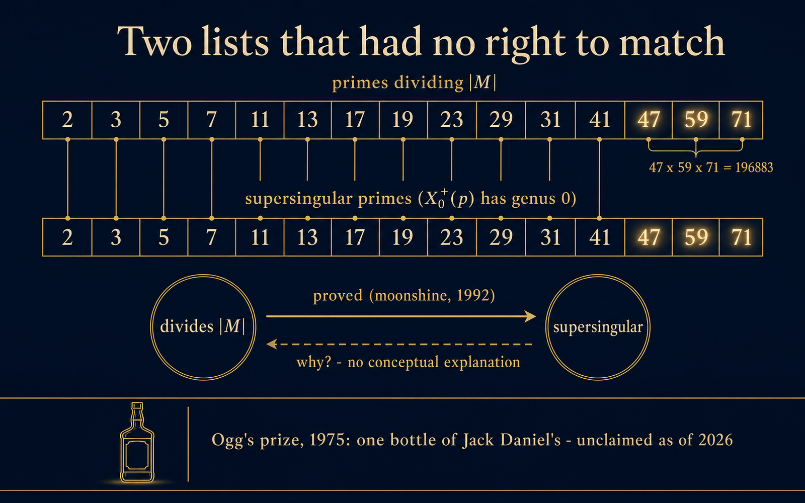
Appendix C concept diagram · Two lists, each computed on its own: the 15 primes dividing (the group-theory side) and the supersingular primes (the number-theory side, of genus zero) are identical to the letter; the solid arrow is the proved direction (divides supersingular), and the reverse direction has to this day no conceptual explanation — that bottle of Jack Daniel’s is still unclaimed. (Made by this channel · mathematical infographic)
What this section is to do. The main text, §3, says: nearly four years before McKay (1975), Ogg had come upon the other half of the riddle — the 15 primes dividing are exactly the “supersingular primes” of number theory. Here the checkable part is checked to the bottom (the list, the product), the uncheckable part is cited honestly, and this “unsolved” item is clearly distinguished from the “unsolved” item of D/E in this episode — they are two different things.
Checkable (checked): , and its 15 prime factors are
the largest three , with product (the crux of EP7 §2). This step is pure arithmetic, checkable.
Statement + citation (Ogg 1975): these 15 primes are exactly the “supersingular primes” — that is, for which the modular curve ( being the Fricke involution) has genus , those primes . Ogg counted out these 15 independently from the side of modular curves, compared them, and found them identical to the letter with the list “divides the order of the Monster”; he offered a bottle of Jack Daniel’s as a reward for an explanation. The proof of the genus-0 classification of = cite Ogg 1975 (this episode does not rebuild it).
Where the name comes from (cited): “supersingular” comes from supersingular elliptic curves — a class of exceptionally special elliptic curves in the world of characteristic (no -torsion points, an anomalously large endomorphism ring). A prime is “supersingular” in the moonshine sense, by the original definition, if: in characteristic , all the supersingular -invariants fall in the prime field ; Ogg 1975 proved that this is equivalent to ” has genus ” — and this appendix uses throughout exactly the latter (computable) characterization. The equivalence of the two statements = cite Ogg 1975, not reproved.
A small example (one stop inside the list and one outside). (on the list): itself has genus , and after taking the quotient by the Fricke involution, has genus — “supersingular” looks at the genus after the quotient. (the first prime not on the list — the list jumps directly from to ): has genus , and at the same time (verified by direct division) — at the first prime where the two lists have a chance to diverge, they give “not on it” in step. The two genus values are cited from Ogg’s 1975 table; this article additionally rechecked them with Riemann–Hurwitz: for the involution quotient , the number of fixed points is taken from the class number formula (when , ; when , ; ; formula cited), and the class numbers , , are computed by counting reduced primitive quadratic forms — substituting gives , , consistent with the cited values (at the stop the answer is known to be , and it is also used to test this algorithm itself).
A full recomputation. The method above need not stop at two stops: for primes , has a closed formula according to and (cited; the two stops and reproduced the values in Ogg’s table), is given by class numbers (class numbers still computed by ourselves), and Riemann–Hurwitz gives immediately. This article used a program, for all 44 primes with , to compute one by one: all 13 primes on the list have , and all the others have , without a single exception — Ogg’s classification in this range is recomputed and rechecked by this article, no longer only cited. (The two ends and the tail are still cited from Ogg 1975 to complete it; a rough intuition: the genus term grows linearly like , the class number term grows only like , so the list will not come back to life far away — this sentence is intuition, not to be used as a proof.) To confirm that this algorithm really is testing something, two controls were done: the two stops and reproduced the values in Ogg’s table; and when, for , the term was deliberately left out, 23 of the 44 primes went wrong immediately ( no longer an integer, or the classification changed).
The boundary of this section. “The two lists are equal” is a checkable fact (both sides can be computed). Moonshine proved one direction: every prime dividing is on Ogg’s list (Monster → genus-0, the Borcherds direction); but the other way round — why every prime on Ogg’s list really divides , why the prime factors of the Monster happen to reach exactly up to — there is no conceptual proof, and that bottle has still not been cleanly claimed by anyone. (That the list itself stops at is not an open case: for the genus of is nonzero, settled by Ogg 1975, and the small example of above is a sample from outside the list; the proved direction also guarantees only that the prime factors of the Monster are , and what hangs open is that they reach exactly the end .) Note: this “unsolved” item is Ogg’s prime coincidence (one number-theoretic direction not closed up), and it is a different matter from the “unsolved” item of Appendices D/E (the genus-0 property of moonshine has been proved by Borcherds, only without a conceptual explanation).
What in this section is computed and what is cited: the product of the prime factors of is a 54-digit decimal number, consistent with ATLAS; the 15 prime factors, the largest three , , , were all checked by program. The class numbers were obtained by counting reduced primitive quadratic forms, and substituting into Riemann–Hurwitz gives , . All 44 primes with were recomputed: the 13 on the list have , and all the others are . Cited and not reproved: the genus formula for , the formula for the fixed points of the Fricke involution, and , Ogg 1975’s classification for and , and the equivalence of the two definitions of “supersingular”.
Appendix D (concepts + cited, not rebuilt) · Vertex operator algebras and the skeleton of Borcherds’s proof
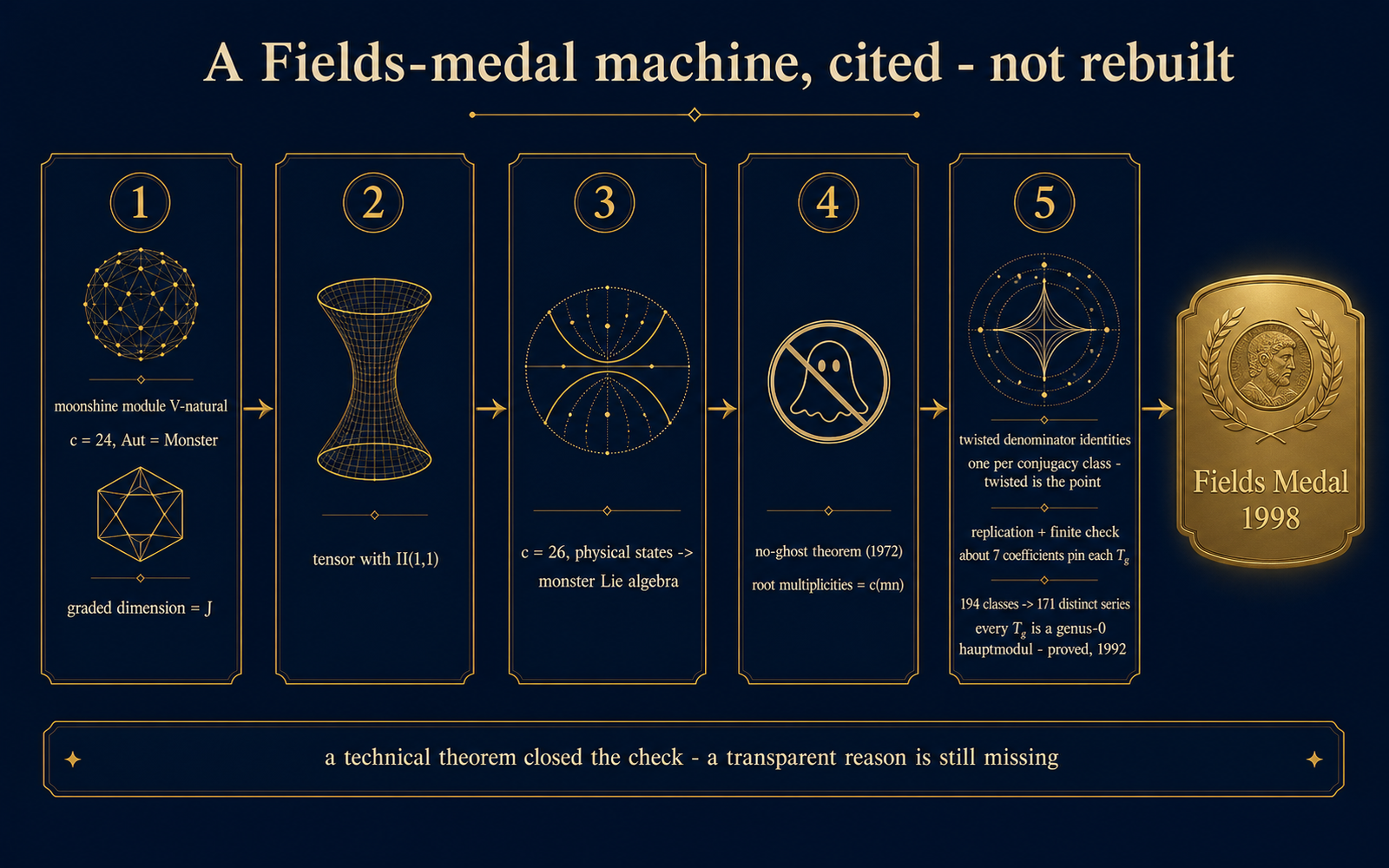
Appendix D concept diagram · From the moonshine module to the theorem: (symmetry group = the Monster, layer-by-layer dimensions = ), via Borcherds’s Monster Lie algebra and the no-ghost theorem, reaches the complete proof of 1992 — the 194 conjugacy classes of the Monster give 171 different McKay–Thompson series, every one genus 0. (Made by this channel · mathematical infographic)
What this section is to do. The main text, §4, says that Frenkel–Lepowsky–Meurman built the “moonshine module” , and Borcherds used it to prove the whole conjecture. Here the skeleton of the proof + its honest boundary are given — this is the only peak in the whole series where “a proof exists, but it cannot be rebuilt in a blog”: Borcherds’s 1992 machinery is Fields Medal work. This appendix only states the structure and points out the key theorems, marking each one clearly as “cited, not rebuilt”, and does not do any formula-by-formula derivation. The main statements were compared against the original literature; which ones were only checked at the level of secondary citation is marked item by item in the sources.
D.1 What a VOA is (semi-formal intuition)
A vertex operator algebra (VOA) is the mathematical axiomatization of 2D chiral conformal field theory: a -graded vector space , each state paired with a “vertex operator” (a formal power series), satisfying axioms such as vacuum, translation, and locality ( commuting up to higher order); a Virasoro element gives and the central charge , and gives the grading. It is exactly the rigorous version of the “operator product expansion” of strings/CFT (Appendix E tells it again from the physics side).
D.2 The moonshine module (FLM 1988, stated, not rebuilt)
This step is the “starting point” of the whole chain. It delivers a concrete object, plus three properties that everything downstream needs: central charge (deciding how much has to be added later to make up ) · automorphism group the Monster (bringing the “group” in) · layer-by-layer dimensions (bringing “the coefficients of ” in). Without this step, Borcherds would have nowhere to start; but it itself proves nothing about — it only puts two things into the same object, and why the conjecture holds remains completely unanswered.
- is the Leech lattice VOA ‘s orbifold: take = the lattice automorphism lifted to ; then
— the -invariant subspace of the untwisted part the -invariant subspace of the unique irreducible -twisted module. (⚠ The orbifold is not as simple as “divide by ”: one must both project onto the -invariants and attach the twisted sector; taking only the invariant subalgebra is not .)
- Central charge (⚠ not 26; 26 is the critical dimension of the string, which comes in only in D.3 below).
- the Monster (FLM, following Griess 1982): acts by construction, and is generated by its weight- space (dimension = the Griess algebra ), and so it equals . is finite precisely because — if there were states of weight , they would generate an affine Kac–Moody current algebra and give an automorphism group of positive dimension (continuous).
- graded dimension = : . ⚠ One place easy to confuse: makes the constant term (the coefficient = the number of states of weight ) equal to , not ; is the constant term of , and it is subtracted to get (constant term ). The leading comes from the vacuum Casimir shift — and are two unrelated numbers, each minding its own business. Weight splits as (untwisted invariant) (twisted invariant) , exactly matching ‘s coefficient and McKay’s (the mental-arithmetic version is in the small example of Appendix E.3).
D.3 The Borcherds skeleton (1992, stated, not rebuilt)
This step is responsible for the whole stretch “from the object to the theorem”. What each of the five steps does is laid out first, before looking at the details — when reading, look at what each step delivers, not what it is called:
| Step | What this step does |
|---|---|
| ① Build | turn into something with a root system, so that “coefficients” have a chance to become “multiplicities” |
| ② no-ghost | the only step that really computes the multiplicities: . The only physics theorem in the whole chain |
| ③ GKM identification | makes step ④ eligible to be written down — not every Lie algebra has a denominator identity |
| ④ Denominator identity | translates the algebraic structure into a product formula for ; only the “twisted” versions give all the , the untwisted one recovers only itself |
| ⑤ Closing up | compresses infinitely many coefficient relations into one finite check |
⟹ Only ② is a physics theorem, only ④ really touches moonshine itself, and ⑤ is the source of “the proof holds but is not transparent” (the honest boundary of D.4 comes exactly from this step).
-
The Monster Lie algebra = the physical states of the vertex algebra of central charge , ( is the lattice VOA of the even unimodular Lorentzian lattice , ). ⚠ One place easy to get wrong: is built on , not the Leech route — the latter gives another algebra (the “fake Monster Lie algebra”, Borcherds 1990, multiplicities ), and the two are not the same object.
-
no-ghost (Goddard–Thorn) ⟹ root multiplicities: the theorem identifies the physical states of momentum with a single graded layer of — and it is an isomorphism of Monster modules, not just equality of dimensions — so the root multiplicity is (). Equivariantly, () become twisted root multiplicities. (Grading convention: uses , uses ; they differ by , and the multiplicity is in both — this article uniformly uses the subscript.)
A small example (putting two concrete numbers into the machine). (a) Take the root : — exactly that layer of D.2, the Griess algebra . The same ; this is the third identity this episode gives it: the left side of McKay’s equation, ‘s coefficient, the multiplicity of a root of the Monster Lie algebra. (b) The first non-trivial coefficient relation given at the lowest order by the denominator identity (item 4 below) is
(This relation is obtained by comparing coefficients in the product formula of item 4 below; the derivation is not redone here; for , recurrences of this kind were first found by Mahler (according to Borcherds 1992 §9). The numerical values on both sides have been substituted with the computed independently by program from the Eisenstein series, and the equation holds.) This is exactly complementary to the boundary line of Appendix B: the identities govern the relations between coefficients and coefficients; how the coefficients decompose into Monster representations (what the multiplicities are) is the matter of “from on, ATLAS must be looked up”. These are two matters.
-
is a generalized (Borcherds–) Kac–Moody algebra (one real simple root of norm + infinitely many imaginary simple roots). ⚠ is an ordinary Lie algebra, not a Lie superalgebra — the “superalgebras” in the title of Borcherds’s paper refers to an auxiliary family of superalgebras, whose exterior-power (super) homology produces the twisted identities.
-
The denominator identity: the Weyl–Kac–Borcherds denominator identity of is exactly the Koike–Norton–Zagier product
(The here is only shorthand for , and has nothing to do with the denoting a prime in Appendix C.) ⚠ Note: this untwisted identity gives only (recovering itself). The “twisted” denominator identities, one for each conjugacy class (equivariant graded traces, one per class), are what give all the — “twisting” is the key, not a footnote. How the three names relate: the product formula is the one for ; writing one for each gives the twisted denominator identities; the coefficient relations they give are the same set as the replication identities that Norton proposed in 1984 for the functions in the Conway–Norton table (Borcherds 1992 §8).
-
Closing up: complete replicability determines each uniquely by its (together with the various powers of ) first coefficients, and then a finite computer check against the functions assigned by Conway–Norton proves that = the genus-0 hauptmodul on the list. Fields Medal, 1998.
D.4 The honest boundary (D)
Genus 0 is proved (not open) — the 194 conjugacy classes of the Monster give 171 different McKay–Thompson series, and each one is proved to equal a genus-0 hauptmodul. But Borcherds closed up by a finite check of coefficients, and gave no conceptual reason for “why genus 0” — Gannon calls it “a computer check — as opposed to a general conceptual argument” (the conceptual gap). Cummins–Gannon (1997, Invent. Math. 129) technically filled in that check with “modular equations ⟹ complete replicability ⟹ hauptmodul”, but that is still a technical theorem, not a transparent principle. The proof exists; the transparent “why” is not there.
Results in this section cited and not reproved: (a) the Goddard–Thorn no-ghost theorem (Goddard–Thorn 1972 / Borcherds’s VOA version); (b) FLM’s construction of (FLM 1988); (c) that satisfies the GKM identification axioms (Borcherds); (d) the Koike–Norton–Zagier product formula; (e) the Lie algebra homology / Adams operation derivation of the twisted identities (Borcherds §8–10, Jurisich); (f) that a Thompson series is uniquely determined by its first 5 coefficients (together with the various powers of ) + the finite check (Borcherds; Cummins–Gannon 1997); (g) the hauptmodul list of Conway–Norton 1979. For each of the items above, this article only states it and gives its source.
Appendix E (conceptual picture) · The string-theory picture
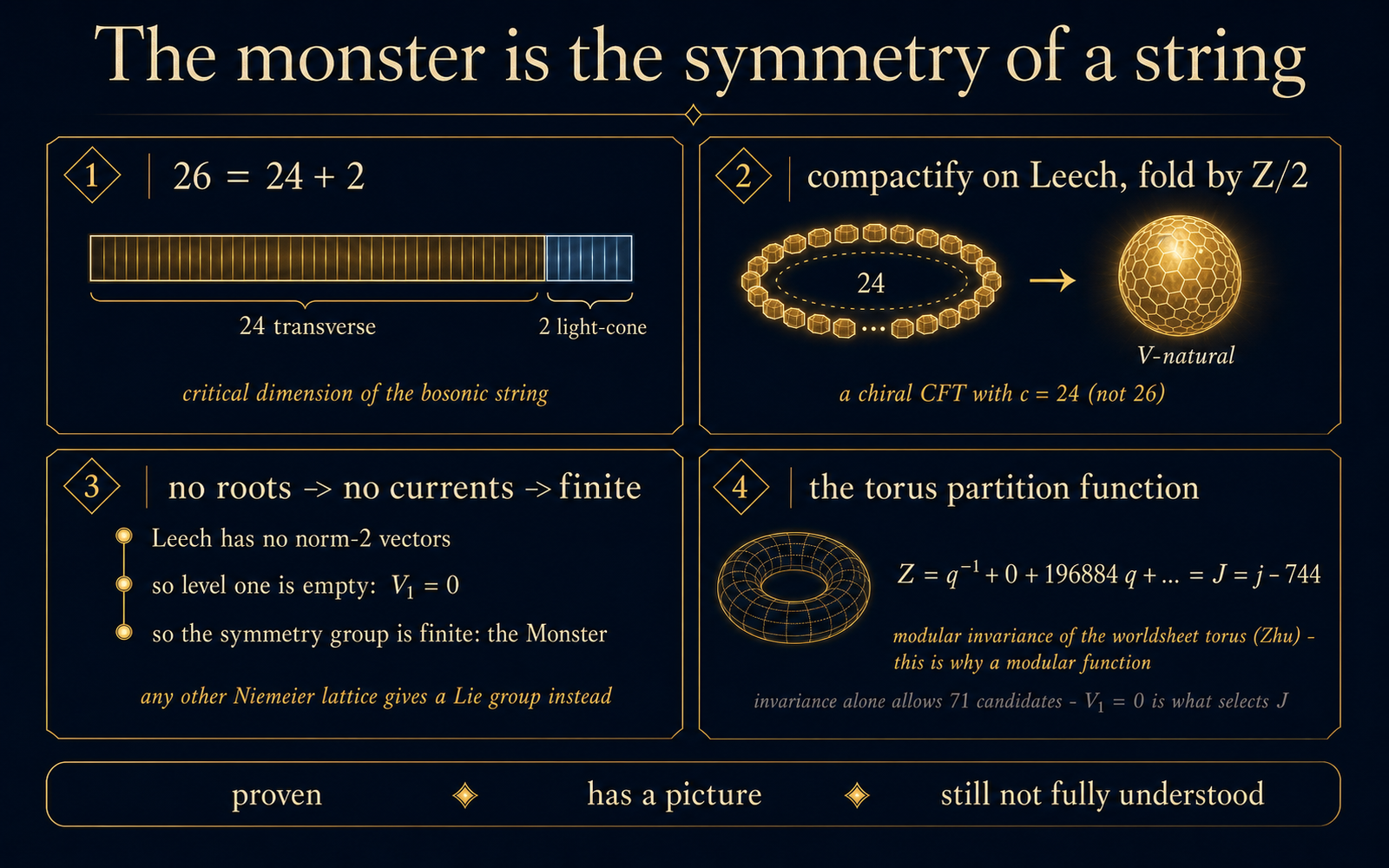
Appendix E concept diagram · The string-theory picture: 24 transverse dimensions compactified on the Leech lattice torus (uniquely rootless ⟹ layer 1 is empty ⟹ the symmetry group can only be finite), and the partition function is exactly ; the modular invariance of the worldsheet torus answers the half “why a modular function”. (Made by this channel · mathematical infographic)
What this section is to do. This is the part of this episode for readers with a theoretical-physics background. It is about physical concepts, not the history of string theory. The goal: to state ” is not an algebra out of thin air — it is a string theory” to a precision that can stand up to a physicist’s nitpicking. The main statements were compared against the original literature (Polchinski / GSW / FLM / Borcherds / Goddard–Thorn / Gannon; which ones were only checked at the level of secondary citation is marked item by item in the sources). Throughout, conceptual statements + key formulas, not formula-by-formula derivation.
What each of the five subsections delivers:
| Delivers | Key point | |
|---|---|---|
| E.1 | where the number comes from: | is the central charge of the string, not of |
| E.2 | the physical identity of = the Leech torus orbifold, | with any lattice that has roots, moonshine cannot be obtained |
| E.3 | partition function , and the answer to “why a modular function” | modular invariance alone does not select — is also needed |
| E.4 | at which step of the proof no-ghost is used | it only supplies the root multiplicities, it does not prove moonshine |
| E.5 | the current state | already proved / there is a picture / not yet understood, three sentences, each saying one thing |
E.1 The critical dimension , and
Under Polyakov (covariant) quantization, the string’s worldsheet is a 2D CFT: free scalars (matter ) + the reparametrization Faddeev–Popov ghosts (weights , ). Weyl (conformal) invariance is a local gauge symmetry, and its anomaly must vanish (equivalently: matter cancels ghost ). Three other roads point to the same number: closure of the light-cone Lorentz algebra (which fixes both and the intercept ) and BRST nilpotency ; these two give just as directly as the cancellation of the Weyl anomaly; the Goddard–Thorn no-ghost theorem, on the other hand, gives an upper bound — for there are no negative-norm states, and is the end point of this range (see E.4). In light-cone gauge one pair is eliminated ( gauge-fixed, solved from the Virasoro constraints), leaving transverse oscillators. So : transverse light-cone.
⚠ Honest boundary (E.1): (a) is not a physical spacetime dimension — the bosonic string is a toy model (it has a tachyon and no spacetime fermions); the critical dimension with physical relevance is the superstring’s ( transverse). (b) That is “forced” holds only for the purely geometric critical string in flat space; add an internal CFT of central charge or a Liouville/linear dilaton mode, and the spacetime dimension can be other than while Weyl invariance still holds. (c) "" should be understood as the light-cone pair that is gauge-fixed + solved from constraints, not as two physical polarizations deleted independently.
E.2 The Leech torus orbifold = (, drawing the line against the string’s )
Compactify the transverse bosons on a 24-dimensional even unimodular lattice, then orbifold away the reflection (), and you get a chiral CFT with — this is the physical face of FLM’s .
⚠ Two places that are easy to state wrongly:
- The central charge is , not . is a holomorphic VOA with , not the string’s worldsheet matter CFT (that has ) — the two are different objects. To recover the critical string from , one must further attach those light-cone directions (the Lorentzian , ) to make up — this is exactly “the two free bosons cancelled” by the Goddard–Thorn functor. So both statements ” has ” and “the string’s transverse CFT is ” are wrong.
- Why exactly Leech. There are 24 even unimodular lattices in 24 dimensions (the Niemeier lattices), and Leech is the only one without roots (minimal norm , no vectors of norm ). It is precisely this “no vectors of norm ” that kills the weight- currents (), handing the automorphism group over to the finite Monster rather than a continuous Lie group. With any Niemeier lattice that has roots, what you get is a CFT with a current algebra, whose automorphism group is a Lie group — not moonshine. So Leech is not a universal property of string theory, only the choice of this one particular compactification. (Detail: there are in fact three cuts here, not one: the candidates for weight originally come by three routes — the Cartan currents on the untwisted side, the root-vector currents () on the untwisted side, and twisted-side states. The first route is -odd and killed by the orbifold projection; the third route has lowest weight above (the twisted vacuum has , and after projection the first contribution is at weight , the ) — these two cuts treat all 24 Niemeier lattices alike. What only Leech lacks is the second route: for a lattice with roots, the -even combinations survive to weight and generate a current algebra. So “rootless” is the cut that keeps the other 23 lattices out at the door — the small example of E.3 computes exactly the same accounting at the weight- layer.)
the Monster; vertex operators = the string’s interaction operators (a VOA is exactly the mathematical axiomatization of this algebra of string operators, Appendix D.1).
E.3 Partition function = , and “why a modular function”
The torus (genus 1) partition function of = the graded character
(The leading comes from the vacuum shift ; the constant term the number of states of weight , so it is , not . In addition, this is the chiral character (holomorphic in only), not the physical non-chiral partition function — is a holomorphic “half”, not an independent unitary local 2D QFT.)
A small example (the same , checked once by two routes of addition). ’s coefficient is the dimension of the layer of the string spectrum. It has two ways of being split up that know nothing of each other:
- The addition on the construction side (CFT sectors, counts cited from FLM): . Untwisted side — two-oscillator states (), states (the norm- vectors of Leech taken in pairs as -invariant combinations; the -projection at the same time eliminates the -odd and ; if a physics reader counts states with nowhere to go, this is where they went); twisted side (one half-integer-mode oscillator × the -dimensional twisted vacuum, after projection).
- The addition on the representation side (the Monster): — the Griess algebra: the trivial representation the smallest faithful representation. The physical identity of McKay’s “+1” is the energy-momentum tensor . The additions have been checked (). The point: the splitting into sectors is not the splitting into Monster representations — the Monster stirs the two sectors together (it is bigger than the symmetry on the lattice side, and bigger exactly here), so the two routes of addition each add up to , yet their details do not match each other. That moonshine “matches, yet no one can say why” can already be seen at this one coefficient.
Modular invariance of the worldsheet ⟷ the modular group of Appendix A. By Zhu’s theorem, a rational, -cofinite, holomorphic VOA with has a character that is a weight- modular function ( makes the -phase ; the -invariance is the content of Zhu). This is the physical/algebraic answer to “why what pops out is a modular function” — the modular invariance of the worldsheet torus leads to exactly the modular group and the class of modular functions of Appendix A.
⚠ A qualification that must be added: modular invariance alone does not select , nor does it bring in the Monster — for all 71 holomorphic VOAs on Schellekens’s list, modular invariance gives only . It is the independent fact of construction (no spin- currents ⟹ no continuous symmetry ⟹ the finite Monster) that selects .
E.4 no-ghost (physics version) and the Monster Lie algebra
The Goddard–Thorn no-ghost theorem (physics version): the physical states of the bosonic string (annihilated by , on the mass shell) have no negative-norm (ghost) states for () — the induced inner product is positive semidefinite. At the critical , the zero-norm states are exactly those orthogonal to the transverse DDF states, they decouple from all amplitudes, and after quotienting out the null states the space is positive definite, isomorphic to the Fock space of transverse oscillators. ⚠ The statement “positive definite for ” is not accurate: in general it is only semidefinite. After quotienting out the zero-norm states, the space obtained is always positive definite; what is special about is that what remains after the quotient is exactly the space spanned by the transverse DDF states (for there are additional longitudinal physical states).
Borcherds wrote it in the language of vertex algebras and used it on (), getting the root multiplicities of the Monster Lie algebra (Appendix D.3). no-ghost supplies only the root multiplicities — it does not construct , does not prove the Monster action, does not prove that is GKM (that needs Borcherds’s identification theorem), and does not prove moonshine. It is a lemma, not the whole proof.
E.5 The current state: already proved, there is a picture, not yet understood
Already proved; there is a physical picture; not yet truly understood.
- Already proved: moonshine is a theorem (the Conway–Norton 1979 conjecture → FLM 1988 built → Borcherds 1992 proved it, Fields 1998), and the genus-0 property is also within what has already been proved; it is not an unsolved problem.
- There is a picture (this half has an answer): is the chiral half of a 2D CFT, and its torus partition function = the modular invariant ; via Zhu, modular invariance is derived from consistency — “why a modular function” really does have an answer.
- Not yet understood (the other half has no answer): (a) why exactly Leech / / the Monster — “the 24-dimensional construction” is a fact, not an explanation (experts still cannot say what the “essential importance” of the Monster lies in, as Gannon has repeatedly pointed out — here his meaning is paraphrased, not quoted word for word); (b) why each is not only modular but a genus-0 hauptmodul (the principal modulus property — Duncan–Griffin–Ono, word for word: “a conceptual explanation for the principal modulus property of monstrous moonshine is yet to be established”).
- ⚠ There are two “genus” here, and they are not about the same thing: “the genus 1 partition function of ” (modular invariance, understood) “why each is a genus-0 group” (the hauptmodul property, not understood).
- The Rademacher sums / 3D chiral gravity program of Duncan–Frenkel is the leading candidate for filling in this conceptual foundation, but it is a conjecture, not a theorem. Gannon: “Moonshine remains mysterious to this day.”
The basis of the statements in this section: /the Weyl anomaly/, the Leech orbifold (), Leech uniquely rootless, /Zhu modular invariance, no-ghost semidefinite/positive definite at criticality, (not Leech = the fake Monster), genus 0 proved but not conceptually explained — the main statements were compared against the following literature, and those checked only at the level of secondary citation are marked item by item in the sources (Polchinski / GSW / FLM 1988 / Borcherds 1992 / Goddard–Thorn 1972 / Gannon / Duncan–Griffin–Ono / Duncan–Frenkel / Zhu 1996 / Schellekens 1993); the entries are in the sources.
Appendix F (checkable) · 194 → 171, class by class
The main text says: the 194 conjugacy classes give 171 different series — inverses take away 22 pairs, and the last step has no mechanism. Here this computation is laid out class by class. The list is Conway–Norton’s own Table 2 in the original (pp. 327–329): they state on p. 314 that the “class” in each row of the table is the union of one or two conjugacy classes — a row in which two classes are merged carries an asterisk at its head. Counting asterisks is counting merges.
The 22 starred rows (in each row two classes share one series; mechanism: mutually inverse, and ):
Three details, exactly the places where readers easily miscount: order 46 appears in two pairs (46AB and 46CD); the letters are not always AB (39CD, 40CD, 56BC, 78BC — because there are classes of the same order that are not merged, listed before them); each starred row reduces the series by only one.
The exceptional one is not among the asterisks. 27A and 27B are two separate rows in Table 2 (centralizer orders and , two different classes), yet they share the same series — this equality is one that Conway–Norton declare separately on p. 310: inverse pairs are equal, “as do the two distinct conjugacy classes of elements of order 27”, and that there are no other equalities. Why this should be so, this article did not find an explanation for. The 22 pair merges are written into the structure of the table; the 23rd merge is written only in one sentence — even the layout is telling you it is an accident.
Three pieces of arithmetic you can count yourself:
| What is counted | How it is counted | Result |
|---|---|---|
| number of rows in the table | single rows starred rows | (= the “number of classes of cyclic subgroups” Gannon counts) |
| conjugacy classes | ✓ | |
| different series | (the two rows 27A/27B share one) | ✓ |
⚠️ There is a trap for anyone counting rows: at the end of Table 2 hang three more rows, 25Z, 49Z, 50Z — Conway–Norton call them “ghost elements” (p. 310 obs (2)): groups of genus 0 that do not correspond to any element of the Monster. Counting them in would give 175 rows. This count excludes these three rows throughout.
The computed/cited boundary of this section: the meaning of the asterisks (two classes merged into one row), the inverse mechanism, the order-27 exception and “no others” — cited (Conway–Norton 1979, pp. 310, 314, 327–329); the transcription of the starred rows, the counting and the three pieces of arithmetic — checked (this article); the pair-by-pair verification that each pair “really is an inverse pair” needs ATLAS power maps, which this article did not do; it is carried by the overall statement on p. 310.
Lean formal verification (2026-09-19)
The places in Appendices A–F that say “checked by program” or “checked” used Python programs and hand derivations. This section checks once again with a different tool: using the theorem prover Lean 4 (4.33.1) and its mathematics library Mathlib, the statements in the appendices that can be formalized were written one by one as Lean theorems and handed to Lean’s kernel to check. Two source files with 57 theorems in total all pass; the axioms used do not go beyond Lean’s three standard axioms (propext, Classical.choice, Quot.sound), there is no sorry, and no shortcut that bypasses the kernel, such as native_decide, is used.
The column “what Lean checked” records only the part that Lean really checked. In many entries what Lean checks is the arithmetic, and the meaning of the numbers themselves comes from elsewhere: Lean can check , but ” is the dimension of the smallest non-trivial representation of the Monster” is not in Lean; premises of this kind are written in the column “where the inputs come from”.
| Appendix | What Lean checked | Where the inputs come from (not checked by Lean) | Method |
|---|---|---|---|
| A.1 | ; generate | — | existing Mathlib theorems |
| A.1 | in , , (the step to , where they are , is not formalized) | — | direct matrix computation |
| A.2 | the appendix’s and Mathlib’s fundamental domain are the same set; existence; uniqueness in the interior (Mathlib’s version is stronger: when both points are in the interior, ) | — | existing Mathlib theorems, with one step added by this article |
| A.2 small example | the matrix of has first row and second row ; | — | exact computation |
| A.3 | ; is nonzero everywhere on ; it has a simple zero at the cusp; ; ‘s coefficient is | — | existing Mathlib theorems (the coefficients of derived by this article from Mathlib’s general formula) |
| A.3 | is invariant under | — | proved by this article |
| A.3 small example, Appendix B | and ; to ; and equal term by term in the first 7 terms | -expansions: those of , given by the first A.3 row above; ‘s general coefficient not formalized separately (only the term checked) | exact multiplication of truncated power series |
| Appendix B | the two sides of the three identities are equal | the Monster dimensions (ATLAS) | exact computation |
| Appendix C | this integer has 54 digits; the 15 numbers are all prime and all divide it; no other prime below 72 divides it; ; | the factorization of (ATLAS) | exact computation |
| Appendix C | the discriminants have reduced primitive quadratic forms respectively | ”number of reduced forms = class number” (classical reduction theory) | enumeration |
| Appendix C full recomputation | 44 primes with ; all integers; exactly for the 13 on the list; when the term is left out, 23 of the 44 go wrong | the genus formula for , the formula for the fixed points of the Fricke involution, Riemann–Hurwitz | exact computation |
| Appendix F | the 22 starred rows are pairwise distinct; , , | the list of starred rows (transcribed from Conway–Norton Table 2) | exact computation |
Seven of the key computations are each paired with a counterexample, to confirm that the check itself will report an error: change to , change the number of forms of discriminant to , change the number of starred rows to , and Lean rejects each.
The parts not formalized: the stabilizers of the two elliptic points in A.2; all of A.4 (the valence formula, a bijection, genus , hauptmodul, , ), because Mathlib currently has no valence formula; the step in A.3 “the product of the truncated power series is the function ‘s -expansion”; the rest of Ogg’s classification in Appendix C ( and ), and the equivalence of the two definitions of “supersingular”; Appendices D, E (which only cite and do not reprove in the first place); the pair-by-pair verification of “mutually inverse” in Appendix F.
Result: within the range checked in the table above, Lean and the numbers and statements of the appendices are not inconsistent in a single place.
Sources
The source book (narrative skeleton)
- Mark Ronan, Symmetry and the Monster, Oxford University Press, 2006 (Prologue / Ch15 “A Monstrous Mystery” / Ch17 “Moonshine”).
Moonshine · observation and conjecture
- Wikipedia · Monstrous moonshine: https://en.wikipedia.org/wiki/Monstrous_moonshine
- MathWorld · Monstrous Moonshine: https://mathworld.wolfram.com/MonstrousMoonshine.html
- J. H. Conway & S. P. Norton, Monstrous Moonshine, Bull. London Math. Soc. 11(3) (1979) 308–339. DOI 10.1112/blms/11.3.308.
- Terry Gannon, Monstrous Moonshine: The First Twenty-Five Years, arXiv:math/0402345.
The moonshine module · vertex operator algebras
- I. B. Frenkel, J. Lepowsky, A. Meurman, A natural representation of the Fischer–Griess Monster with the modular function J as character, PNAS 81(10) (1984) 3256–3260.
- I. Frenkel, J. Lepowsky, A. Meurman, Vertex Operator Algebras and the Monster, Academic Press, 1988.
The proof · string theory · the Fields Medal
- R. E. Borcherds, Monstrous moonshine and monstrous Lie superalgebras, Invent. Math. 109 (1992) 405–444. DOI 10.1007/BF01232032 (author’s copy: https://math.berkeley.edu/~reb/papers/monster/monster.pdf).
- P. Goddard & C. B. Thorn, Compatibility of the dual Pomeron with unitarity and the absence of ghosts in the dual resonance model, Phys. Lett. B 40 (1972) 235–238 (the no-ghost theorem).
- Borcherds, Gowers, Kontsevich, and McMullen Receive Fields Medals, Notices of the AMS 45(10), November 1998, 1358–1360: https://www.ams.org/notices/199810/comm-fields.pdf
- Simon Singh’s interview with Borcherds (“I was over the moon…”), The Guardian, 1998-08-28 (the original text is kept on the author’s own website: https://simonsingh.net/media/articles/maths-and-science/interview-with-richard-borcherds/); reprinted (edited) in Mail & Guardian 1998-09-11: https://mg.co.za/article/1998-09-11-moonshine-and-the-mathematician/ (the MacTutor biography of Borcherds cites the same sentence).
- Marcus du Sautoy, Finding Moonshine, 2008 (US edition title Symmetry) — the source of McKay’s line “I was a bit peeved really”; this article cites it at second hand from Lieven Le Bruyn, the McKay-Thompson series: http://www.neverendingbooks.org/the-mckay-thompson-series/ , without having seen the page in the original book.
After the book (2006–2026)
- Eguchi, Ooguri, Tachikawa (the Mathieu moonshine observation), arXiv:1004.0956 (2010) — “The reason is yet a mystery”.
- Gannon, Much ado about Mathieu, arXiv:1211.5531 (2012).
- Gaberdiel, Hohenegger, Volpato, Symmetries of K3 sigma models, arXiv:1106.4315 (2011) — the source of “no K3 model carries a faithful M24 action” (the constraint that the symmetry group ⊆ the Co₁ side).
- Cheng, Duncan, Harvey (the umbral moonshine conjecture), arXiv:1204.2779 (2012); the Niemeier lattice version arXiv:1307.5793 (2013).
- Duncan, Griffin, Ono, Proof of the Umbral Moonshine Conjecture, Res. Math. Sci. 2:26 (2015), arXiv:1503.01472.
- Duncan, Mertens, Ono, Pariah moonshine, Nature Communications 8:670 (2017).
- Paquette, Persson, Volpato (a physical derivation of genus 0), arXiv:1601.05412 (2016); the self-description of the mathematical level as a sketch is in arXiv:1701.05169 (J. Phys. A, 2017).
Ogg · supersingular primes
- A. P. Ogg, Automorphismes de courbes modulaires, Séminaire Delange-Pisot-Poitou, Tome 16 (1974-1975), no. 1, Exposé no. 7, 8 p. MR 417184, Zbl 0336.14006. https://www.numdam.org/item/SDPP_1974-1975__16_1_A4_0/ (The original sentence offering the reward is in Remarque 1; the criterion Ogg gave is or ; he himself did not list those 15 numbers.)
- Wikipedia · Supersingular prime (moonshine theory) / Monstrous moonshine.
- J. Duncan & K. Ono, The Jack Daniels Problem, arXiv:1411.5354.
People
- John McKay: https://en.wikipedia.org/wiki/John_McKay_(mathematician) · John H. Conway: https://mathshistory.st-andrews.ac.uk/Biographies/Conway/ · Simon P. Norton: https://en.wikipedia.org/wiki/Simon_P._Norton · Richard Borcherds: https://mathshistory.st-andrews.ac.uk/Biographies/Borcherds/ · Andrew Ogg: https://en.wikipedia.org/wiki/Andrew_Ogg
Cited in the appendices (each entry is marked with the level to which it was checked: [registered] = the record was retrieved from Crossref or arXiv on 2026-10-09 and compared item by item; [secondary] = copied from the reference list of another work, the original not seen)
- R. L. Griess, Jr., The friendly giant, Invent. Math. 69 (1982) 1–102. DOI 10.1007/BF01389186. [registered]
- J. G. Thompson, Some numerology between the Fischer–Griess Monster and the elliptic modular function, Bull. London Math. Soc. 11(3) (1979) 352–353; in the same volume, Finite groups and modular functions, 347–351. [registered]
- The character table of the Monster by B. Fischer, D. Livingstone, M. P. Thorne: an unpublished computation, as described on p. 308 of Conway–Norton 1979. [secondary]
- J. H. Conway, R. T. Curtis, S. P. Norton, R. A. Parker, R. A. Wilson, Atlas of Finite Groups, Clarendon Press, Oxford, 1985. [secondary: Borcherds 1992, reference [14]]
- OEIS A001379, Degrees of irreducible representations of Monster group M: https://oeis.org/A001379 ; A007267, A007241, A101558 (the coefficients of ). [registered]
- J.-P. Serre, A Course in Arithmetic, Springer, New York, 1973. DOI 10.1007/978-1-4684-9884-4. [registered]
- T. M. Apostol, Modular Functions and Dirichlet Series in Number Theory, Springer, New York, 1990. DOI 10.1007/978-1-4612-0999-7. [registered]
- H.-V. Niemeier, Definite quadratische Formen der Dimension 24 und Diskriminante 1, J. Number Theory 5(2) (1973) 142–178. DOI 10.1016/0022-314X(73)90068-1. [registered]
- J. H. Conway, N. J. A. Sloane, Sphere Packings, Lattices and Groups, Springer, New York, 1999. DOI 10.1007/978-1-4757-6568-7. [registered]
- R. Fricke, Die elliptischen Funktionen und ihre Anwendungen, Teubner, 1922. [secondary: OEIS A007267]
- S. Ramanujan, Modular equations and approximations to π, in Collected Papers of Srinivasa Ramanujan (ed. G. H. Hardy et al.), pp. 23–39, AMS Chelsea, 2000. [secondary: OEIS A007241]
- R. E. Borcherds, The monster Lie algebra, Adv. Math. 83(1) (1990) 30–47. DOI 10.1016/0001-8708(90)90067-W. [registered]
- Y. Zhu, Modular invariance of characters of vertex operator algebras, J. Amer. Math. Soc. 9(1) (1996) 237–302. DOI 10.1090/S0894-0347-96-00182-8. [registered]
- A. N. Schellekens, Meromorphic c = 24 conformal field theories, Commun. Math. Phys. 153(1) (1993) 159–185. DOI 10.1007/BF02099044; arXiv:hep-th/9205072. [registered]
- C. J. Cummins, T. Gannon, Modular equations and the genus zero property of moonshine functions, Invent. Math. 129(3) (1997) 413–443. DOI 10.1007/s002220050167. [registered]
- T. Gannon, The algebraic meaning of genus-zero, arXiv:math/0512248 (2005). [registered]
- J. F. R. Duncan, M. J. Griffin, K. Ono, Moonshine, Res. Math. Sci. 2 (2015). DOI 10.1186/s40687-015-0029-6; arXiv:1411.6571. [registered]
- J. F. R. Duncan, I. B. Frenkel, Rademacher sums, moonshine and gravity, Commun. Number Theory Phys. 5(4) (2011) 849–976. DOI 10.4310/CNTP.2011.v5.n4.a4; arXiv:0907.4529. [registered]
- The product formula : for the proof see Borcherds 1992 §7, Lemma 7.1 (called the product formula for the j function in the text, unattributed); “Koike–Norton–Zagier” is the customary name, and this article did not check the attribution to the three against a primary source.
- Replication identities: S. P. Norton, More on moonshine, in Computational Group Theory, Academic Press, 1984, pp. 185–193 (proposed); M. Koike, On replication formula and Hecke operators, Nagoya University preprint (proof). [secondary: Borcherds 1992, references [28], [25]]
- J. Polchinski, String Theory, Cambridge University Press, 1998. DOI 10.1017/CBO9780511816079. [registered]
- M. B. Green, J. H. Schwarz, E. Witten, Superstring Theory, Cambridge University Press. [registered]
Epigraph
- This sentence comes from Schopenhauer’s Parerga und Paralipomena, Volume II, §76 (1851). The chapter epigraph of Chapter 17 of Ronan’s book prints the English of this sentence, attributed to Schrödinger; this article and the video use the English wording printed in Ronan’s book and its Chinese translation, with the attribution changed back to Schopenhauer.